Amplitude Damping: Why Energy Loss Is Not a Random Bit Flip
Model qubit energy loss with Kraus operators, test it in NumPy, and see why a random X gate cannot reproduce amplitude damping on every input.
A qubit in its excited state can lose energy and fall to its ground state. If a simulator replaces that process with a random X gate, it may get one population measurement right while predicting the wrong behavior for other inputs.
Amplitude damping is the standard simple channel for this kind of relaxation. Its most useful lesson is that quantum noise is not always a lottery over ordinary gates.
Start with a direction of energy flow
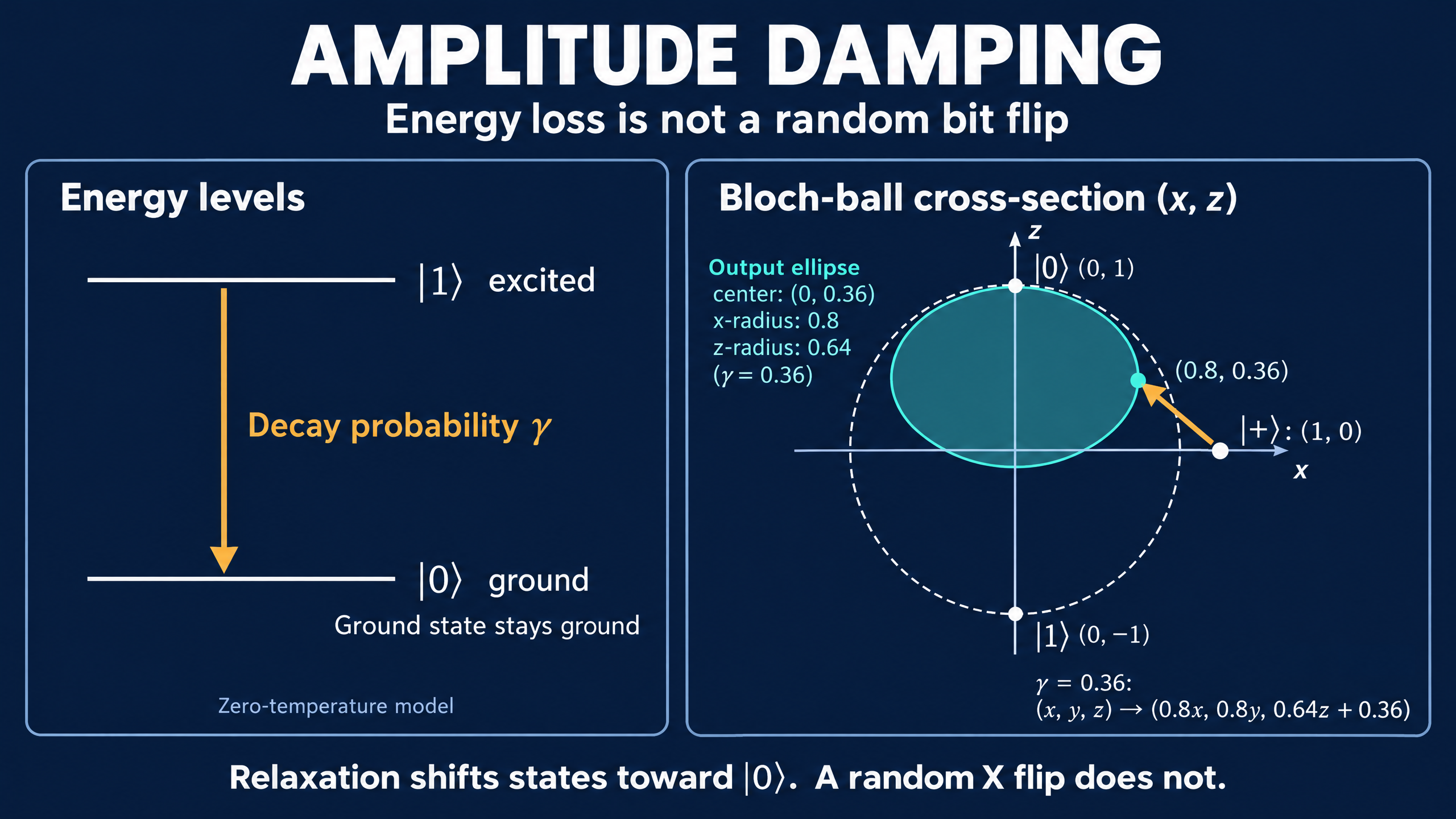
Use the ordered basis |0>, |1>, with |0> the ground state and |1> the excited state. Let gamma be the probability that a qubit initially in |1> decays during the modeled interval. In the zero-temperature model, there is no competing upward excitation:
|0><0| stays |0><0|
|1><1| becomes gamma |0><0| + (1-gamma) |1><1|
For exponential relaxation with a constant lifetime T1, the interval t corresponds to:
gamma = 1 - exp(-t/T1)
This means gamma is a probability, not a decay rate. The excited-state survival probability is 1-gamma. IBM Quantum Learning's noise lesson derives this relation and the channel below.
A random X error with probability gamma produces the same output as amplitude damping if the input is |1>. But it also sends |0> upward with that probability. Amplitude damping leaves |0> alone. One test input is not enough to identify a noise process.
Two Kraus operators, one physical channel
To handle superpositions and mixed states consistently, write the channel using Kraus operators:
K0 = [[1, 0], [0, sqrt(1-gamma)]]
K1 = [[0, sqrt(gamma)], [0, 0]]

E(rho) = K0 rho K0† + K1 rho K1†
The dagger means conjugate transpose. These operators satisfy K0†K0 + K1†K1 = I, which ensures that the channel preserves total probability.
K1 is the energy-loss branch. For a general input, its probability is gamma times the excited-state population, not gamma regardless of the state. K0 is the complementary branch. Crucially, K0 is not the identity: it reduces the excited-state amplitude relative to the ground-state amplitude.
This is why a picture of "do nothing or apply X" fails. Even the branch associated with no emitted excitation changes the relative amplitudes of a superposition. Kraus operators describe a possible decomposition of the process, not necessarily a measurement that the experimenter actually performs, and that decomposition is not unique.
For a density matrix with populations a and b and coherence c, the result is:
rho    = [[a, c], [c*, b]]
E(rho) = [[a + gamma b,       sqrt(1-gamma) c],
          [sqrt(1-gamma) c*, (1-gamma) b]]
Here c* is the complex conjugate of c. Relaxation changes both populations and coherence. Pure dephasing, by contrast, leaves these populations unchanged.
A small NumPy implementation
The following code applies the full channel to a density matrix. It sums the unnormalized Kraus contributions. It does not condition on a jump record or simulate individual experimental shots.
import numpy as np

def amplitude_damp(rho, gamma):
    if not 0 <= gamma <= 1:
        raise ValueError("gamma must be a probability")
    K0 = np.diag([1, np.sqrt(1 - gamma)]).astype(complex)
    K1 = np.array([[0, np.sqrt(gamma)], [0, 0]], dtype=complex)
    return K0 @ rho @ K0.conj().T + K1 @ rho @ K1.conj().T

gamma = 0.36
plus = np.ones((2, 2), dtype=complex) / 2  # |+><+|
states = {
    "ground": np.diag([1, 0]).astype(complex),
    "excited": np.diag([0, 1]).astype(complex),
    "plus": plus,
    "mixed": np.eye(2, dtype=complex) / 2,
}

print("state     P(1)    |rho01|")
for name, rho in states.items():
    out = amplitude_damp(rho, gamma)
    assert np.isclose(np.trace(out), 1)
    assert np.linalg.eigvalsh(out).min() >= -1e-12
    print(f"{name:7}  {out[1, 1].real:.3f}   {abs(out[0, 1]):.3f}")

X = np.array([[0, 1], [1, 0]], dtype=complex)
flipped_plus = (1 - gamma) * plus + gamma * X @ plus @ X
print(f"random X on plus: P(1)={flipped_plus[1, 1].real:.3f}, "
      f"|rho01|={abs(flipped_plus[0, 1]):.3f}")
Output:
state     P(1)    |rho01|
ground   0.000   0.000
excited  0.640   0.000
plus     0.320   0.400
mixed    0.320   0.000
random X on plus: P(1)=0.500, |rho01|=0.500
For |+>, amplitude damping gives the matrix [[0.68, 0.40], [0.40, 0.32]]. A random X leaves |+><+| unchanged, because |+> is an X eigenstate. The two models therefore disagree even though they matched for the excited-state population test.
A common implementation mistake is to normalize each Kraus contribution separately and then add the results. That discards the branch weights. For the unconditional channel, simply sum K rho K† as above.
The Bloch ball moves toward the ground state
With the convention rho = (I + xX + yY + zZ)/2, the ground state sits at z = +1. Amplitude damping acts as:
x -> sqrt(1-gamma) x
y -> sqrt(1-gamma) y
z -> (1-gamma) z + gamma
There is both contraction and a shift. For gamma = 0.36, the input |+> has Bloch coordinates (1, 0, 0) and moves to (0.8, 0, 0.36). The ground state remains fixed.
The maximally mixed state I/2 also moves, becoming [[0.68, 0], [0, 0.32]] in this example. A channel that preserves the identity is called unital. Amplitude damping with gamma greater than zero is not unital. Any probability mixture of unitary gates is unital, so no such mixture can reproduce this channel exactly on every input.
In the complete-damping limit gamma = 1, every input ends in |0><0|. Noise can therefore make a qubit more pure by relaxing it toward a known ground state. That is not the same as preserving the unknown quantum information it originally carried.
What this model leaves out
The simple channel assumes relaxation toward the ground state, without thermal excitation or additional pure dephasing. Real devices can have all of those effects, along with leakage and control errors.
The Qiskit Aer amplitude-damping API includes a generalized version with an equilibrium excited-state population. Setting that population to zero recovers the model used here. The NumPy example is a channel calculation, not a forecast of a particular processor's performance.
When building a noise model, test more than one input. Checking the excited state, the ground state, and a superposition reveals whether you modeled directed energy loss or merely a random change of computational-basis labels.