Approximate QFT: Why Matching Counts Is Not Enough
Dropping small controlled rotations can shorten a quantum Fourier transform. A three-qubit NumPy example shows why identical measurement counts do not prove the approximation preserved the state.
Imagine optimizing a quantum Fourier transform by deleting one controlled rotation. You simulate the exact and shortened circuits, measure their outputs in the computational basis, and get matching probability distributions.
Did the optimization preserve the quantum state? Not necessarily. It may have changed relative phases that this measurement cannot see.
That is a useful trap to understand before using the approximate quantum Fourier transform, or AQFT. The approximation deliberately trades some accuracy for fewer gates. The important question is whether its error matters to the algorithm that uses it, not just whether one histogram looks unchanged.
Why remove rotations at all?
The standard n-qubit QFT circuit uses Hadamards, controlled phase rotations, and a final reversal of the wire order. Its controlled phases become progressively smaller as the qubits involved get farther apart.
Write a one-qubit phase gate as
P(angle) = diag(1, exp(i*angle)).
Its controlled version applies that phase only when both participating qubits are 1. The rotation family often called R_k has angle 2*pi / 2**k. Thus R_2 has angle pi/2, R_3 has angle pi/4, and later members have smaller angles.
A common AQFT construction omits controlled rotations below a chosen cutoff. The standard exact circuit has a quadratic number of controlled phases. Keeping only m nearby partners per wire reduces that count to O(n*m). The cutoff still has to satisfy an error budget; fixed m does not guarantee arbitrary accuracy as n grows.
This is a deterministic change to the intended unitary, not a model of random hardware noise. Fewer gates may help on hardware, but the benefit has to outweigh the approximation error.
A three-qubit circuit with one missing gate
Use the basis order |q0 q1 q2>, where q0 is the most-significant bit. Define the positive-sign QFT by
Q[y, x] = exp(2*pi*i*x*y/8) / sqrt(8).
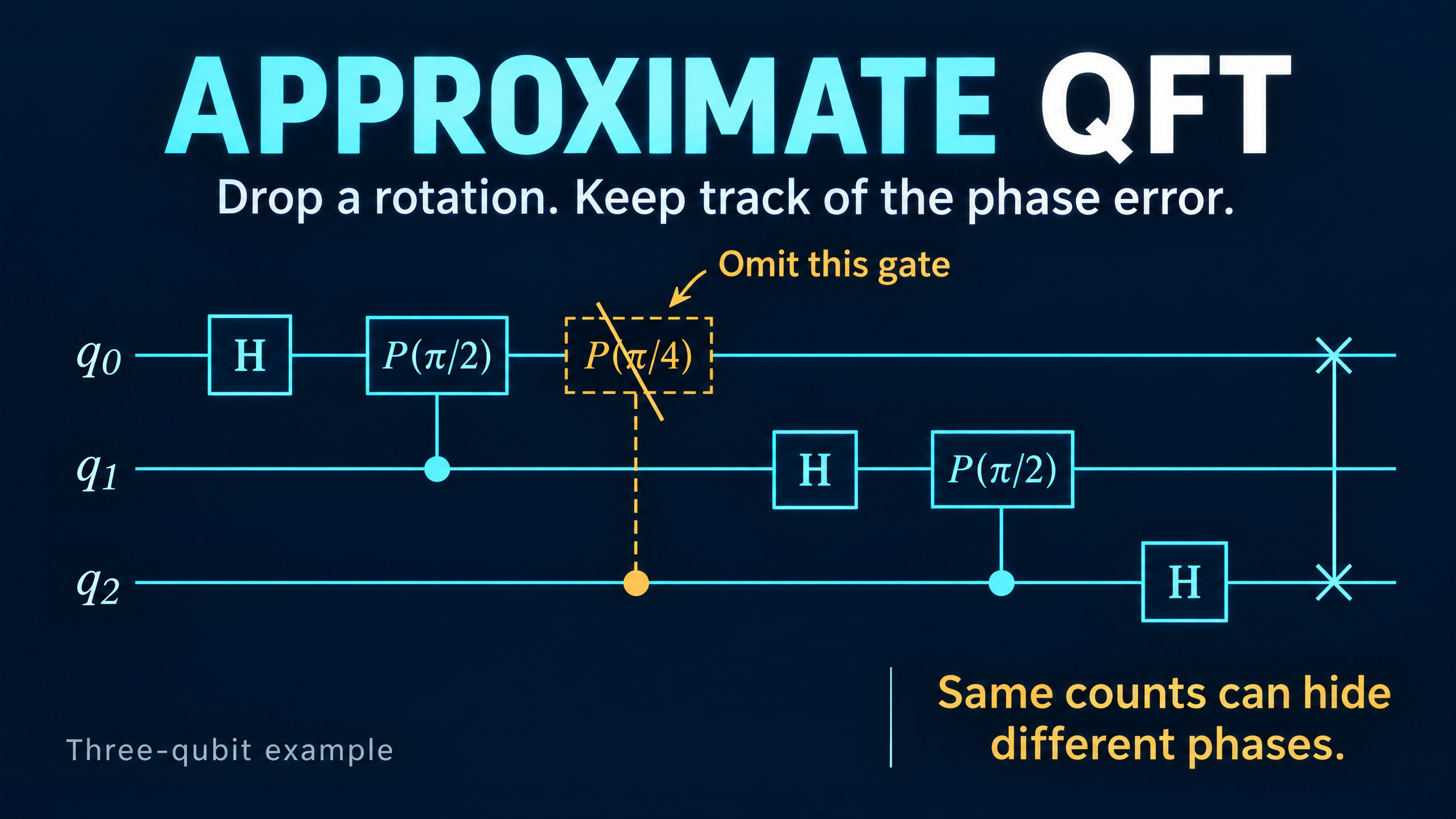
The circuit in the cover performs these operations in time order:
- H on q0.
- Controlled P(pi/2), with q1 controlling q0.
- Controlled P(pi/4), with q2 controlling q0.
- H on q1.
- Controlled P(pi/2), with q2 controlling q1.
- H on q2.
- SWAP q0 and q2.
For the approximate circuit, delete only step 3. Keep both pi/2 rotations and the final SWAP. Stating the final wire reversal matters because otherwise a correct result can look wrong simply through reversed bit order.
We use a tiny circuit to expose the error clearly. Pi/4 is not an extremely small angle, so this is not a recommendation to use that cutoff in a larger application.
Same probabilities, different states
Start from |001>, which represents integer 1. After the exact circuit, the output is the product state
|-> tensor (|0> + i|1>)/sqrt(2) tensor (|0> + exp(i*pi/4)|1>)/sqrt(2).
After the truncated circuit, it is
|-> tensor (|0> + i|1>)/sqrt(2) tensor |+>.
Only the final factor differs. Its relative phase has changed, and a global phase cannot remove that difference.
Both states give probability 1/8 for every computational-basis string. No number of measurements in that basis alone can distinguish these two ideal output distributions.
Their squared-overlap fidelity, however, is
F = abs(<exact|approx>)**2 = cos(pi/8)**2,
which is about 0.853553. Their pure-state trace distance is sqrt(1 - F), about 0.382683. The latter characterizes their optimal measurement distinguishability; it is not the difference between the two Z-basis histograms, which is zero here.
Check the phases, not just the counts
This NumPy example constructs the exact QFT matrix and the derived approximate output above. It is a state-comparison demonstration, not a general circuit compiler.
As an additional phase-sensitive test, apply the exact inverse QFT to the approximate output. If that output were the exact Fourier state, the inverse would return |001> with certainty. Instead, the return probability is the fidelity.
import numpy as np

z = np.array([1, 0], dtype=complex)
o = np.array([0, 1], dtype=complex)
minus = (z - o) / np.sqrt(2)
plus = (z + o) / np.sqrt(2)
y = np.arange(8)
Q = np.exp(2j * np.pi * np.outer(y, y) / 8) / np.sqrt(8)
exact = Q[:, 1]  # QFT of |001>, with q0 most significant
approx = np.kron(np.kron(minus, (z + 1j*o) / np.sqrt(2)), plus)

F = abs(np.vdot(exact, approx))**2
D = np.sqrt(max(0.0, 1 - F))
back = Q.conj().T @ approx
same_counts = np.allclose(np.abs(exact)**2, np.abs(approx)**2)

assert np.allclose(Q.conj().T @ Q, np.eye(8))
assert np.isclose(np.vdot(approx, approx).real, 1)
assert np.isclose(F, np.cos(np.pi / 8)**2)
assert np.isclose(abs(back[1])**2, F)
assert same_counts

print(f"Fidelity: {F:.10f}")
print(f"Trace distance: {D:.10f}")
print("Same Z-basis probabilities:", same_counts)
print(f"Exact-inverse return probability: {abs(back[1])**2:.10f}")
print(f"Omitted-gate operator norm: {2*np.sin(np.pi/8):.10f}")
Expected output:
Fidelity: 0.8535533906
Trace distance: 0.3826834324
Same Z-basis probabilities: True
Exact-inverse return probability: 0.8535533906
Omitted-gate operator norm: 0.7653668647
The exact inverse is a diagnostic here, not a proposed cost-saving production step. Using the approximate circuit's own inverse would merely test that the approximate circuit is reversible. It would not prove that the circuit implements the intended QFT.
A simple bound on deletion error
For one controlled phase CP(angle), its operator-norm difference from the identity is
norm(CP(angle) - I) = 2*abs(sin(angle/2)).
This follows because its diagonal entries are 1, 1, 1, and exp(i*angle). Surrounding the omitted gate with identical unitary operations on both circuits preserves this norm difference.
For our single deletion, the full circuits therefore differ in operator norm by 2*sin(pi/8), about 0.765367. This is a worst-case circuit-level quantity, not the fidelity loss 1-F for our selected input.
For several deleted rotations, a telescoping expansion and the triangle inequality give a safe bound: add the individual gate-norm errors. Since 2*abs(sin(angle/2)) <= abs(angle), the sum of the omitted absolute angles is a simpler upper bound. Such bounds can be loose, but they make the accuracy budget explicit.
Input-specific tests are still useful. For example, deleting these controlled rotations does not change the output on |000>. Passing that test alone says little about other inputs.
What to test before accepting the shortcut
An AQFT is useful when the saved gate cost is worth its effect on the surrounding algorithm. In a small simulation, compare state fidelities or the full unitary, not only computational-basis counts. In an application, also test the quantity the algorithm actually needs, such as phase-estimation success probability.
The lesson is not that small rotations must always be kept. It is that matching one measurement distribution does not certify a matching quantum transformation. An optimization can be sensible and still require a phase-sensitive test.
Further reading
Coppersmith's original approximate Fourier-transform report introduces the approximation in the context of quantum factoring.
Reducing T-count and T-depth in approximate quantum Fourier transform discusses controlled-rotation truncation and the separate costs of fault-tolerant gate synthesis. Our example studies deletion error only, not rotation-synthesis error.