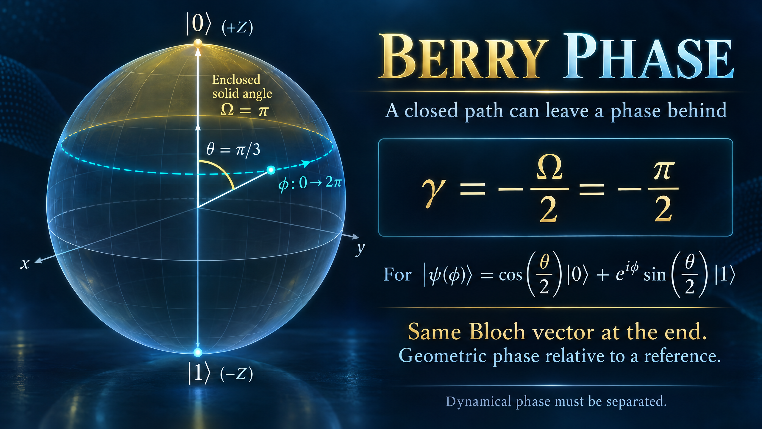
Berry Phase: A Closed Qubit Path Can Leave a Phase Behind
A qubit can return to the same Bloch vector after a loop and still acquire a geometric phase. Calculate a latitude loop, test gauge invariance, and separate geometry from dynamical phase.
Take a qubit around a closed path on the Bloch sphere. Its final Bloch vector can match its initial one exactly, while the evolving state vector acquires a phase that remembers the route.
This is not a loophole in the rule that global phase is unobservable. The phase becomes measurable only relative to another coherent branch. The interesting part is that one contribution depends on the geometry of the path rather than the time spent traveling along it.
That contribution is the Berry phase. A simple latitude loop makes both its calculation and its numerical pitfalls easy to see.
Specify the path and the sign
Consider the normalized qubit states
|psi(phi)> = cos(theta/2)|0> + exp(i*phi)*sin(theta/2)|1>.
Their Bloch vectors are
(sin(theta)*cos(phi), sin(theta)*sin(phi), cos(theta)).
Hold theta fixed and increase phi from 0 to 2*pi. The vector traces a latitude circle, counterclockwise when viewed from the positive Z axis. The north-pole cap bounded by this loop has solid angle
Omega = 2*pi*(1 - cos(theta)).
For the state convention above and this direction of traversal, the geometric phase is
gamma = -Omega/2 = -pi*(1 - cos(theta)), modulo 2*pi.
At theta equal to pi/3, Omega is pi and gamma is -pi/2. Reversing the path reverses the sign, modulo 2*pi. Specifying the state and orientation matters when comparing formulas from different sources.
Where the phase comes from
For our smooth, periodic choice of state vectors, the Berry phase can be written as
gamma = i * integral_0^(2*pi) <psi(phi)|d/dphi psi(phi)> dphi.
The inner product is i*sin(theta/2)**2. Multiplying by the leading i and integrating gives -2*pi*sin(theta/2)**2, which is the solid-angle formula above.
The chosen representative |psi(phi)> returns to itself at the endpoint. That does not mean the physically evolving state accumulates no phase. These vectors specify the instantaneous direction in Hilbert space; the actual evolution can carry an additional phase factor along that direction.
Geometry is not the entire time evolution
One physical realization uses a Hamiltonian
H(t) = -(Delta/2) * n(t) dot (X, Y, Z),
where Delta is positive and n(t) is the unit Bloch vector on the loop. The state we wrote is the ground eigenstate, with energy -Delta/2.
Starting in that eigenstate and changing n(t) smoothly and sufficiently slowly keeps the system near the corresponding instantaneous eigenspace. In units where hbar equals 1, the accumulated dynamical phase for duration T is
delta = -integral E(t) dt = +Delta*T/2.
The total phase is delta plus gamma in the adiabatic limit. Changing the traversal time changes delta. Traversing the same oriented loop with a different slow time schedule leaves gamma unchanged.
A finite-speed implementation can depart from the adiabatic approximation. The geometric formula alone does not bound those errors or make a gate automatically robust to noise.
Calculate the loop from neighboring overlaps
Instead of differentiating state vectors, sample N points around the loop and form
W = product_j <psi_j|psi_(j+1)>, with psi_N = psi_0.
Then -arg(W) approaches the Berry phase as the sampling becomes fine. At finite N, it is a discretized approximation to the smooth latitude loop. The minus sign agrees with our earlier convention.
The closing overlap from the last sample back to the first is essential. It also makes the calculation insensitive to arbitrary phase choices for the sampled vectors.
A reproducible NumPy example
The code below excludes the repeated endpoint, then closes the cycle using np.roll. It applies an independent random phase to every sampled state and checks that the resulting loop phase is unchanged modulo 2*pi.
import numpy as np

rng = np.random.default_rng(7)
theta = np.pi / 3
exact = -np.pi * (1 - np.cos(theta))

print("N      gamma_approx (rad)       wrapped gauge difference")
for n in (32, 128, 512, 2048):
    phi = 2 * np.pi * np.arange(n) / n  # endpoint excluded
    psi = np.column_stack((
        np.full(n, np.cos(theta / 2), dtype=complex),
        np.exp(1j * phi) * np.sin(theta / 2),
    ))
    norms = np.linalg.norm(psi, axis=1)
    assert np.allclose(norms, 1.0)
    overlaps = np.sum(np.conj(psi) * np.roll(psi, -1, axis=0), axis=1)
    assert np.all(np.abs(overlaps) > 0)
    gamma = -np.angle(np.prod(overlaps))

    alpha = rng.uniform(0, 2 * np.pi, size=n)
    psi_g = psi * np.exp(1j * alpha)[:, None]
    overlaps_g = np.sum(np.conj(psi_g) * np.roll(psi_g, -1, axis=0), axis=1)
    gamma_g = -np.angle(np.prod(overlaps_g))
    wrapped_difference = np.angle(np.exp(1j * (gamma_g - gamma)))
    assert np.allclose(np.exp(1j * gamma_g), np.exp(1j * gamma), atol=1e-12)
    print(f"{n:<6d} {gamma: .15f}       {wrapped_difference: .3e}")

assert np.isclose(exact, -np.pi / 2)
print(f"gauge invariant: True")
print(f"exact target:    {exact:.15f} rad")
Output from the tested run:
N      gamma_approx (rad)       wrapped gauge difference
32     -1.567002244691471       -6.661e-16
128    -1.570559732047842       -4.441e-16
512    -1.570781541710875       -2.887e-15
2048   -1.570795402735299        6.661e-16
gauge invariant: True
exact target:    -1.570796326794896 rad
The phase converges toward -pi/2. The tiny gauge differences are floating-point noise, and their last digits can vary across numerical environments.
This program computes geometry from prescribed states. It does not simulate a timed Hamiltonian, prove adiabaticity, or perform a sequence of physical measurements.
Why arbitrary state phases cancel
Replacing each sampled vector by exp(i*alpha_j)|psi_j> multiplies its overlap with the next vector by
exp(i*(alpha_(j+1) - alpha_j)).
Those factors cancel around the closed cycle. If you omit the closing link, they do not generally cancel. This is useful when working with numerical eigensolvers, which can return different arbitrary eigenvector phases at neighboring parameter values.
The wrapped comparison in the code also matters: phases differing by 2*pi are physically equivalent even if their raw floating-point numbers look far apart.
What an experiment would need to compare
Measuring the final isolated qubit cannot reveal an overall phase. An interference experiment must compare the loop with a coherent reference and account for the dynamical contribution.
For example, conceptually compare the moving ground-state path with a reference held at the initial Hamiltonian for the same duration and with the same energy. Their dynamical phases then match in this ideal model, while only the moving branch encloses the loop. Preparing and recombining such branches requires additional control; our overlap calculation does not implement that protocol.
The takeaway is a distinction worth keeping: returning to the same Bloch vector fixes the final qubit state up to phase, but an interferometer can still remember the path.
Further reading
ETH Zurich notes on Berry's phase derive the dynamical and geometric contributions and the spin-half solid-angle result.
The geometric-phase overview provides broader context and explains why interference is needed to observe the phase.