Deferred Measurement: Turn Feed-Forward into Coherent Control
Replace mid-circuit measurement and feed-forward with coherent control. A NumPy example shows which outputs agree and why the intermediate states can still differ.
A measurement in the middle of a quantum circuit can choose what happens next. Measure a qubit, read a classical bit, then apply a gate only if that bit is one. That is ordinary feed-forward.
There is often another way to obtain the same requested outputs: keep the qubit unmeasured, use it as a quantum control, and read it out later. This is the deferred measurement principle. The important part is not simply moving a measurement symbol to the right. The operation that depended on its result must change too.
Start with a small conditional program
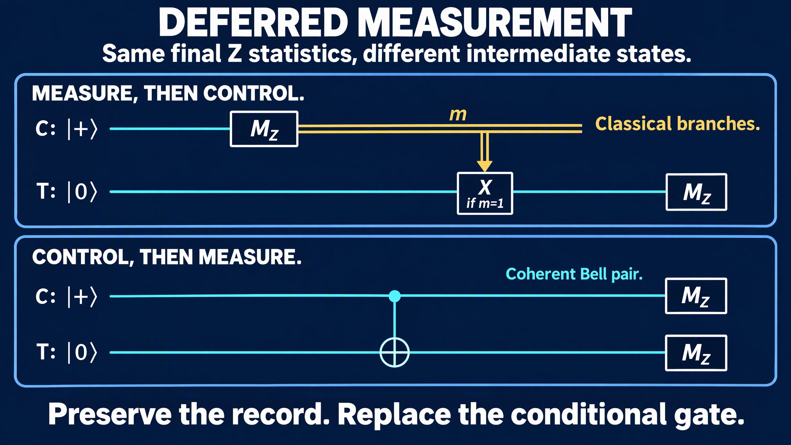
Call the first qubit C and the second qubit T. Prepare C in |+> and T in |0>. Consider this program:
- Measure C in the computational, or Z, basis and call the result m.
- If m is one, apply X to T. Otherwise, do nothing.
- Measure T in the Z basis.
The output pair (m, t) is 00 or 11, each with probability one half. No entangled state needs to survive after the first measurement: the two branches can be understood as a classical random bit choosing the target's state.
Now replace the first two steps with a CNOT from C to T. Measure both qubits in Z at the end. The same two output pairs appear with the same probabilities.
Before that final measurement, however, the deferred circuit holds the Bell state (|00> + |11>)/sqrt(2). Matching the requested output statistics does not mean the two programs have identical intermediate quantum states.
Why the replacement works
Let P0 = |0><0| and P1 = |1><1| on C, and let U act on T. An operation controlled coherently by C is
V = P0 tensor I + P1 tensor U
It applies I in the zero branch and U in the one branch, without first converting the control into a classical result.
For an arbitrary joint input density matrix rho, measuring C and then applying the conditional gate gives
rho_early = K0 rho K0^dagger + K1 rho K1^dagger
K0 = P0 tensor I
K1 = P1 tensor U
Here C retains the measured basis value, so it also represents the classical branch label. This expression averages over both results; it is not a state conditioned on one selected outcome.
Instead apply V first. If C is then measured in Z, averaging over that measurement gives
rho_late = sum over b in {0,1} of
           (Pb tensor I) V rho V^dagger (Pb tensor I)
Because (Pb tensor I)V equals Kb, rho_late equals rho_early. The individual branch operators match too, so the outcome probabilities and the target states conditioned on each result agree. This argument does not require the input qubits to start uncorrelated.
The simple construction assumes the control is preserved until its eventual Z readout. Operations on the target alone can still occur in the meantime. Reusing or resetting the control needs a more careful construction that preserves its earlier measurement record elsewhere.
Check the states, not just the histogram
The following example needs only NumPy. It uses basis order 00, 01, 10, 11, with C on the left and T on the right. These are exact ideal density-matrix calculations, not sampled hardware results.
import numpy as np

I = np.eye(2, dtype=complex)
X = np.array([[0, 1], [1, 0]], dtype=complex)
P0 = np.diag([1, 0]).astype(complex)
P1 = np.diag([0, 1]).astype(complex)

plus = np.array([1, 1], dtype=complex) / np.sqrt(2)
zero = np.array([1, 0], dtype=complex)
psi = np.kron(plus, zero)
rho = np.outer(psi, psi.conj())

K0 = np.kron(P0, I)
K1 = np.kron(P1, X)
V = K0 + K1  # CNOT: C controls an X on T

# Measure C, then apply X to T in the m=1 branch.
early = K0 @ rho @ K0.conj().T + K1 @ rho @ K1.conj().T

# Defer the measurement by using coherent control.
coherent = V @ rho @ V.conj().T
readout_projectors = [np.kron(P0, I), np.kron(P1, I)]
late = sum(M @ coherent @ M for M in readout_projectors)

XX = np.kron(X, X)
def expectation(state, observable):
    return float(np.trace(state @ observable).real)

print("Early Z probabilities:", np.diag(early).real)
print("Deferred Z probabilities:", np.diag(coherent).real)
print("Equal after control readout:", np.allclose(early, late))
print(f"Early <XX>: {expectation(early, XX):.1f}")
print(f"Coherent <XX>: {expectation(coherent, XX):.1f}")
Output:
Early Z probabilities: [0.5 0.  0.  0.5]
Deferred Z probabilities: [0.5 0.  0.  0.5]
Equal after control readout: True
Early <XX>: 0.0
Coherent <XX>: 1.0
The first two lines agree, but the last two do not. Measuring both qubits in X would reveal a difference between the early mixture and the still-coherent Bell state. That is a different experiment from the original program, which reads C in Z. Once the deferred control is actually measured in Z, its branch coherence is gone and the averaged state matches the early version.
This is why checking only final bit counts can hide an important change in a circuit's meaning.
A useful equivalence is not a free optimization
Software can use this principle to simulate some dynamic circuits with ordinary controlled gates. The PennyLane deferred-measurements documentation describes exactly that substitution. It also notes extra-wire requirements when a measured wire is subsequently reused or reset.
That resource cost matters. A classical record can outlive a measured qubit that is reset for another job. A coherent replacement must keep the record available in a quantum system instead. Controlled operations also have their own gate and connectivity costs. Conversely, real mid-circuit measurement introduces readout and feed-forward overheads. Neither version is automatically faster or less noisy on every device.
The equivalence can also be used in the opposite direction. In a dynamic-circuit implementation of the quantum Fourier transform followed by measurement, suitable quantum controls become measurements and classical feed-forward. The final-measurement condition is essential: this is not a claim that the dynamic circuit supplies the same unmeasured QFT output state for arbitrary later processing.
When moving a measurement, ask three questions: where will its record live, what replaces the conditional operation, and which outputs must stay the same? Those questions turn a slogan about delaying readout into a reliable circuit transformation.