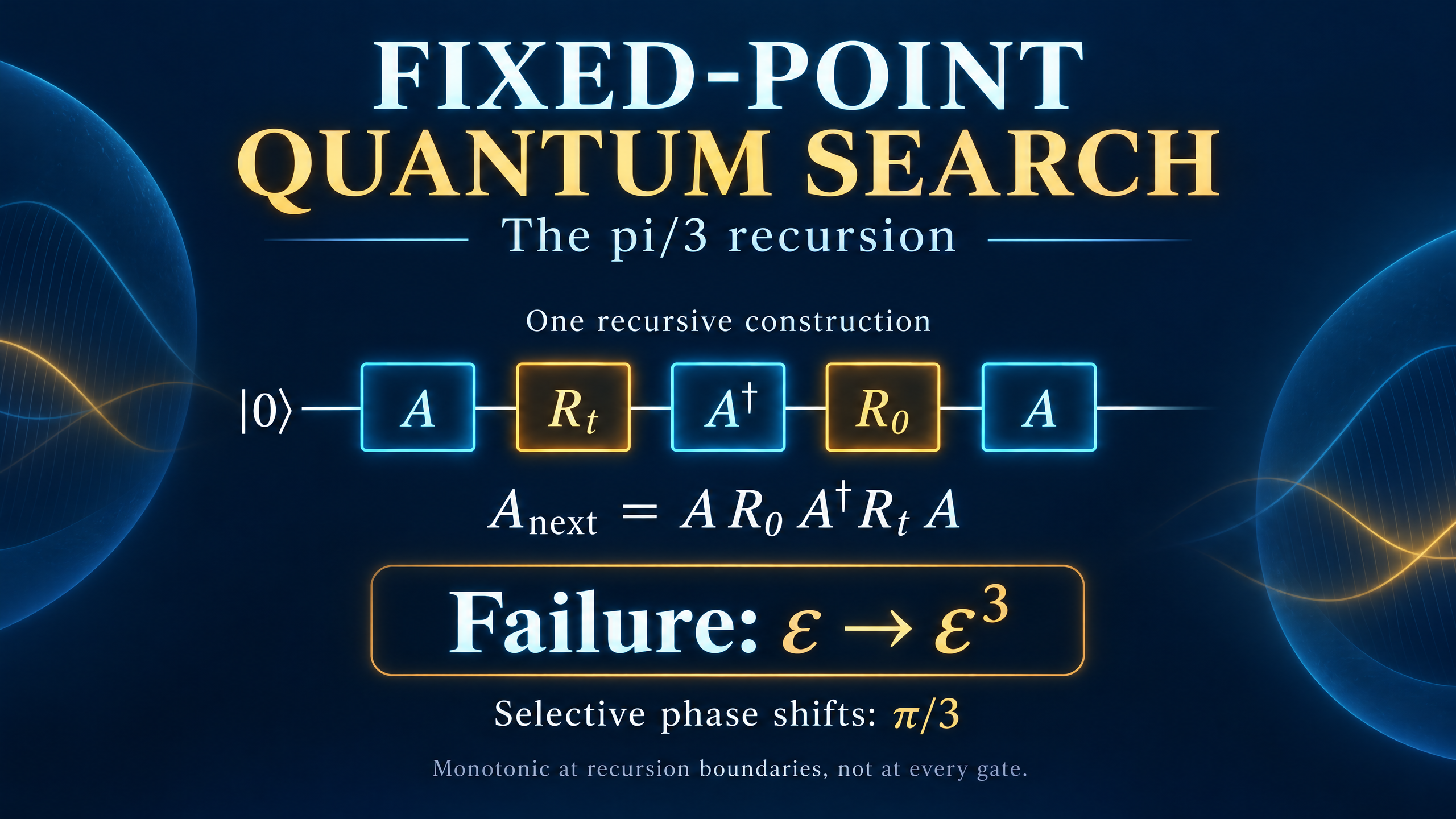
Fixed-Point Quantum Search: Cube the Failure Without Overshooting
The pi/3 search recursion turns failure probability epsilon into epsilon cubed. Test it in NumPy, see why success improves at recursion boundaries, and account for the growing circuit cost.
Ordinary amplitude amplification has a timing problem. Apply the Grover rotation enough times and the success probability rises. Keep going past the useful stopping point and it can fall again.
A different construction replaces the usual selective sign changes with phase shifts of pi/3. Its promise is striking: if a preparation circuit fails with probability epsilon, one composite construction fails with probability epsilon cubed.
This is Grover's original pi/3 fixed-point search scheme. It avoids overshooting at recursion boundaries, but it pays for that property with a growing circuit. The cost is part of the story, not a footnote.
A preparation circuit and two selective phases
Let A be a unitary preparation circuit. Start from |0>, and call |1> the target in a small two-dimensional example. Suppose
p = abs(<1|A|0>)**2 and epsilon = 1 - p.
Define z = exp(i*pi/3), and use two selective phase operations:
R0 = diag(z, 1) applies phase z to the source state |0>.
Rt = diag(1, z) applies phase z to the target state |1>.
These are not measurements. They leave the probabilities unchanged when applied alone, but change the relative phases that later operations can turn into interference.
The improved preparation is
A_next = A R0 A† Rt A.
Operators act on state vectors from right to left. The actual circuit therefore applies A, then Rt, then A-dagger, then R0, then A. The cover shows that chronological order.
For a larger search problem, Rt must mark the desired target state or subspace through a suitable predicate. A small matrix that phases |1> does not magically supply an oracle for an unknown answer.
Why the failure gets cubed
For this composite construction, the amplitude in the unwanted direction gains the factor
z + p*(z - 1)**2.
The choice pi/3 makes the algebra unusually simple:
(z - 1)**2 = -z.
The factor is therefore z*(1 - p) = z*epsilon. Since z has unit magnitude, the failure amplitude shrinks in magnitude by epsilon. Its probability was epsilon, so its new probability becomes
epsilon * epsilon**2 = epsilon**3.
Thus
p_next = 1 - (1 - p)**3.
For 0 < p < 1, this is strictly larger than p. If p is already one, it stays one. If p is zero, the construction cannot create a missing initial overlap.
This is a probability guarantee. It does not promise that every intermediate gate increases success, nor that the target amplitude acquires a prescribed phase.
Recurse the circuit, not the measured output
Set A_0 equal to the original preparation. At the next level, replace every occurrence of A in the construction with A_k:
A_(k+1) = A_k R0 A_k† Rt A_k.
Each level defines a new preparation circuit, evaluated from the same source state |0>. It is not a loop that measures success after each individual gate, and it is not repeated application of one unchanged unitary to the previous output.
If the initial success probability is p0, the exact ideal result is
p_k = 1 - (1 - p0)**(3**k).
The error decreases across these completed recursion levels. That qualification matters: unitary evolution has not become a dissipative process that pulls every possible state toward the same attractor.
A small NumPy experiment
Use a real rotation as A_0, with p0 equal to 0.2. The two-by-two representation is enough to expose the interference identity. It is a transparent toy example, not a demonstration of finding an unknown item in a large database.
The matrix element A[1, 0] is the amplitude for reaching |1> from |0>. Notice that the code rebuilds A, not a state vector carried between measurements.
import numpy as np

p0 = 0.2
zeta = np.exp(1j * np.pi / 3)
R0 = np.diag([zeta, 1.0])
Rt = np.diag([1.0, zeta])
A = np.array([[np.sqrt(1-p0), -np.sqrt(p0)],
              [np.sqrt(p0), np.sqrt(1-p0)]], dtype=complex)

print("level  success       base-A uses")
previous = 0.0
for k in range(4):
    p = abs(A[1, 0])**2
    expected = 1 - (1-p0)**(3**k)
    assert np.allclose(A.conj().T @ A, np.eye(2))
    assert np.isclose(p, expected)
    assert p >= previous - 1e-12
    print(f"{k:5d}  {p:.10f}  {3**k:11d}")
    previous = p
    if k < 3:
        A = A @ R0 @ A.conj().T @ Rt @ A
Expected output:
level  success       base-A uses
    0  0.2000000000            1
    1  0.4880000000            3
    2  0.8657822720            9
    3  0.9975821484           27
The last level has success above 99.7 percent in this noiseless example. But it requires 27 uses of the base preparation or its inverse, not three inexpensive repetitions.
The cost behind the reassuring convergence
Each new level contains two forward copies and one inverse copy of the previous preparation. If B_k counts uses of the base A_0 or A_0-dagger, then
B_0 = 1, B_(k+1) = 3*B_k, so B_k = 3**k.
Counting a call to the target phase operation or its inverse as one selective-phase query gives (3**k - 1)/2 such calls. Expanding an inverse circuit also introduces inverse phase gates; those are not free missing operations.
For small p0, reaching a constant success probability requires 3**k on the order of 1/p0. This original pi/3 scheme therefore does not retain ordinary amplitude amplification's quadratic query advantage, whose relevant scaling is 1/sqrt(p0).
For a target failure tolerance delta, the condition is
(1 - p0)**(3**k) <= delta.
You do not need the exact p0 to define the recursion. You do need information such as a reliable lower bound on p0 to choose a depth with a guaranteed tolerance. Without any positive overlap guarantee, no finite depth provides uniform high success for arbitrarily tiny p0.
What this does and does not solve
The construction assumes coherent access to A and its inverse, plus the selective phase operations. A-dagger is not an instruction to undo an unknown noise channel. Extra depth can introduce additional hardware errors, so the ideal monotonicity is not an unconditional experimental guarantee.
It is also important not to generalize this cost penalty to every fixed-point search method. Later work by Yoder, Low, and Chuang achieves fixed-point error guarantees with optimal quadratic query scaling using a different phase design. This tutorial is about the simpler original pi/3 recursion.
The useful lesson is that avoiding overshoot and minimizing query cost are different design goals. The failure-cubing identity gives a clean, testable example of how carefully chosen phases improve a preparation, and why that improvement must be weighed against the circuit used to obtain it.
Further reading
Grover's original report, A different kind of quantum search, derives the pi/3 construction, the cubed failure probability, and its recursive expansion.
Fixed-point quantum search with an optimal number of queries explains the original scheme's cost limitation and introduces a different construction that preserves the quadratic speedup.