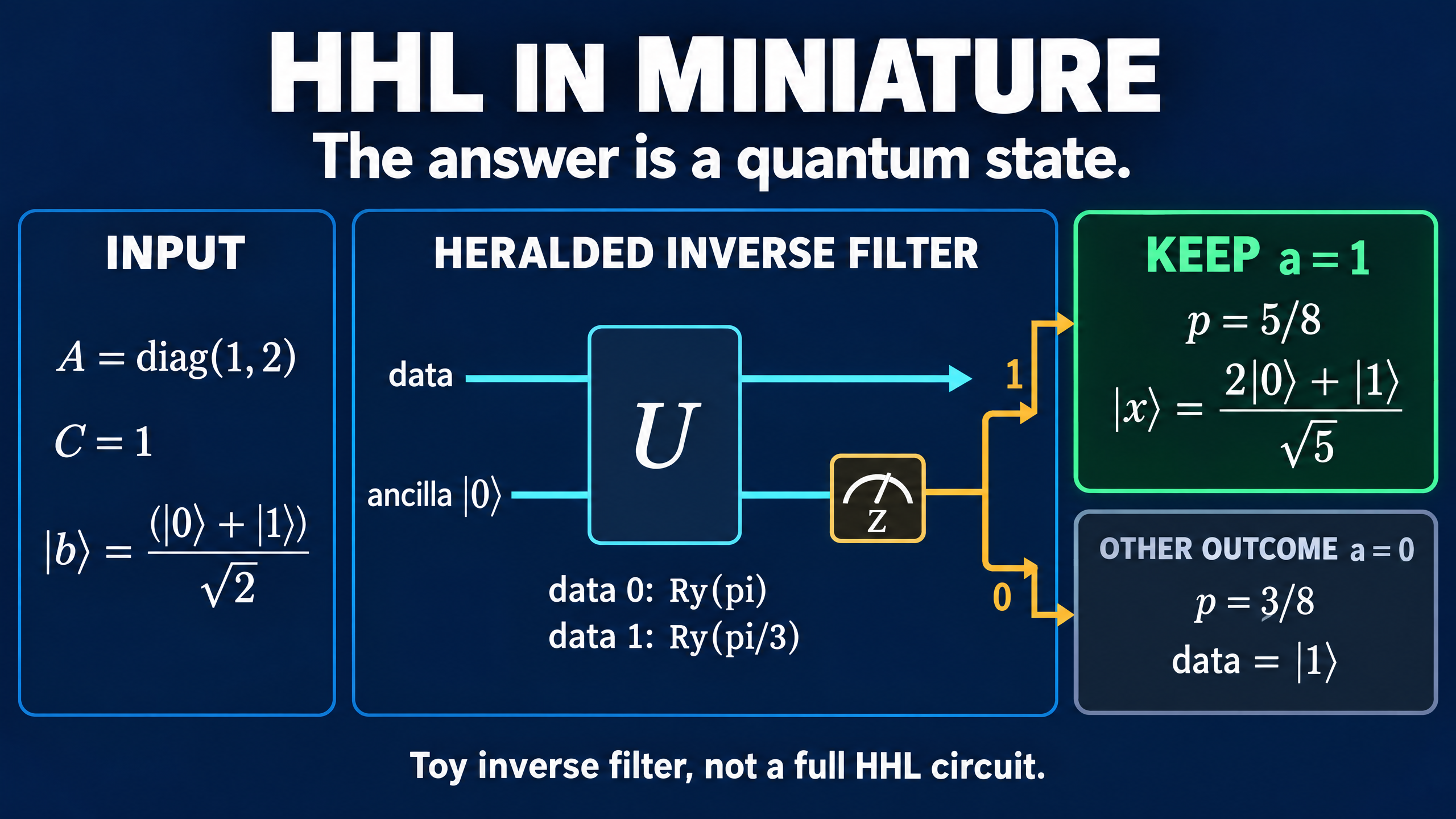
HHL in Miniature: Why a Quantum Linear Solver Returns a State
See how HHL turns inverse eigenvalues into a heralded solution state, test a two-qubit NumPy example, and understand the costs hidden by a state-vector answer.
Ask a classical linear solver for x in Ax = b and you expect a list of numbers. The Harrow-Hassidim-Lloyd algorithm, usually called HHL, offers a different kind of answer: a quantum state whose amplitudes are proportional to the solution.
That change in output is not a minor implementation detail. It determines what you can read out, which costs matter, and whether a claimed speedup answers the problem you actually wanted to solve.
We can see the essential mechanism with one data qubit and one success flag, without pretending that a tiny hard-coded circuit is a complete HHL implementation.
The answer has to be normalized
Take a positive-definite Hermitian matrix A and a normalized input state |b>. Write its spectral decomposition as
A = sum_j lambda_j |u_j><u_j|
|b> = sum_j beta_j |u_j>
All eigenvalues lambda_j are positive in the case considered here. Applying the inverse would give
A^(-1)|b> = sum_j (beta_j / lambda_j) |u_j>
But that vector generally does not have norm one. The solution state is instead
|x> = A^(-1)|b> / ||A^(-1)|b>||
It preserves the direction of the solution vector, not its overall scale. If the original classical b was not normalized, its norm is another piece of bookkeeping. The original HHL paper explicitly targets information about the solution rather than printing every entry of a classical vector.
Put the inverse in a successful branch
Multiplying amplitudes by different inverse eigenvalues is generally not a unitary operation on the data alone. HHL uses an ancilla to make this transformation part of a larger unitary operation.
Choose a positive constant C no larger than the smallest eigenvalue. For an eigenvector |u_j>, the ideal eigenvalue-dependent rotation produces
|u_j>|0>_a -> |u_j>[
    sqrt(1 - C^2/lambda_j^2)|0>_a
    + (C/lambda_j)|1>_a
]
Measuring the ancilla and retaining outcome a = 1 leaves the unnormalized data vector C A^(-1)|b>. Normalizing this branch gives |x>. Its success probability is
p_success = C^2 ||A^(-1)|b>||^2
The other outcome is a different transformation, not generally the desired solution. Both outcomes count toward the experimental cost. A technical analysis of HHL postselection gives these two ancilla branches explicitly.
In a full HHL workflow, phase estimation coherently encodes eigenvalue information, that information controls the rotation, and the eigenvalue register is uncomputed before the final ancilla readout. Finite eigenvalue precision introduces approximation error. None of those steps amounts to measuring an eigenvalue and then classically choosing a single eigenvector.
A two-qubit example you can check
Use this particularly simple system:
A = diag(1, 2)
|b> = (|0> + |1>) / sqrt(2)
C = 1
The successful branch applies diag(1, 1/2) to |b>. After normalization,
|x> = (2|0> + |1>) / sqrt(5)
p_success = 5/8
The inverse favors the component with the smaller eigenvalue. This is amplitude reweighting, not a measurement that somehow reveals both solution entries at once.
Here is an exact NumPy simulation of the ancilla rotation and postselection. The eigenvalues and eigenvectors are already known, so the rotations are hard-coded in the computational basis. This deliberately skips phase estimation and is not a general HHL solver. Tensor-product order is data first, ancilla second.
import numpy as np

A = np.diag([1.0, 2.0])
b = np.array([1.0, 1.0]) / np.sqrt(2)
C = 1.0

# Each block is Ry(2*arcsin(C/lambda)), acting on the ancilla.
U = np.zeros((4, 4))
for j, eigenvalue in enumerate(np.diag(A)):
    s = C / eigenvalue
    c = np.sqrt(1 - s * s)
    rotation = np.array([[c, -s], [s, c]])
    block = slice(2 * j, 2 * j + 2)
    U[block, block] = rotation

assert np.allclose(U.T @ U, np.eye(4))
joint = U @ np.kron(b, np.array([1.0, 0.0]))

# Rows are data values; columns are ancilla outcomes.
branch = joint.reshape(2, 2)[:, 1]
p_success = float(np.vdot(branch, branch).real)
solution = branch / np.sqrt(p_success)

reference = np.linalg.solve(A, b)
reference /= np.linalg.norm(reference)
fidelity = abs(np.vdot(reference, solution)) ** 2

print(f"Success probability: {p_success:.6f}")
print("Solution amplitudes:", np.round(solution, 6))
print("Conditional Z probabilities:", np.round(abs(solution) ** 2, 6))
print(f"State fidelity: {fidelity:.6f}")
assert np.isclose(fidelity, 1.0)
Output:
Success probability: 0.625000
Solution amplitudes: [0.894427 0.447214]
Conditional Z probabilities: [0.8 0.2]
State fidelity: 1.000000
The remaining probability, 3/8, belongs to ancilla outcome zero. In this particular example that failure branch leaves the data in |1>. Ignoring the flag and mixing the two branches does not produce the pure solution state.
These are exact ideal-state calculations, not hardware measurements or sampled shot counts. The classical solve is only a reference for this tiny example, not evidence of a computational advantage.
What can you learn by measuring it?
Among successful preparations, a Z-basis measurement returns 0 with probability 0.8 and 1 with probability 0.2. It does not return the pair of amplitudes 0.894427 and 0.447214.
Those probabilities alone also miss relative signs and phases. For instance, changing the plus sign in |x> to a minus sign leaves its Z probabilities unchanged. Other measurement settings are needed to distinguish them.
A useful output might instead be an expectation value of a chosen observable, or a state passed into another quantum subroutine. Recovering a general N-entry solution as a classical list requires additional work and cannot retain a total runtime that is merely logarithmic in N, since writing the list alone takes N entries.
The condition number is part of the bill
For a positive-definite Hermitian matrix, the condition number is kappa = lambda_max/lambda_min. Small eigenvalues make inversion more sensitive to errors and can make successful state preparation costly.
For example, rescale a spectrum into [1/kappa, 1] and choose C = 1/kappa. The ideal success probability lies between 1/kappa^2 and 1, depending on |b>. An input entirely on the largest-eigenvalue eigenvector reaches the lower endpoint; one on the smallest reaches the upper endpoint. This is a bound on this postselection step, not the full algorithm's runtime. Amplitude amplification can improve the success overhead, but adds coherent circuit work.
A serious resource estimate must also include preparing |b>, accessing A in a form that supports efficient simulation, resolving its spectrum accurately enough, and estimating the final observable. Sparse matrices with suitable access are a standard HHL setting, not a guarantee that loading an arbitrary spreadsheet is cheap.
The right question is therefore more precise than whether a quantum computer can solve linear equations. Can it prepare the required solution state, with the needed accuracy and total cost, and can the information you want be extracted without asking it to print the whole vector?