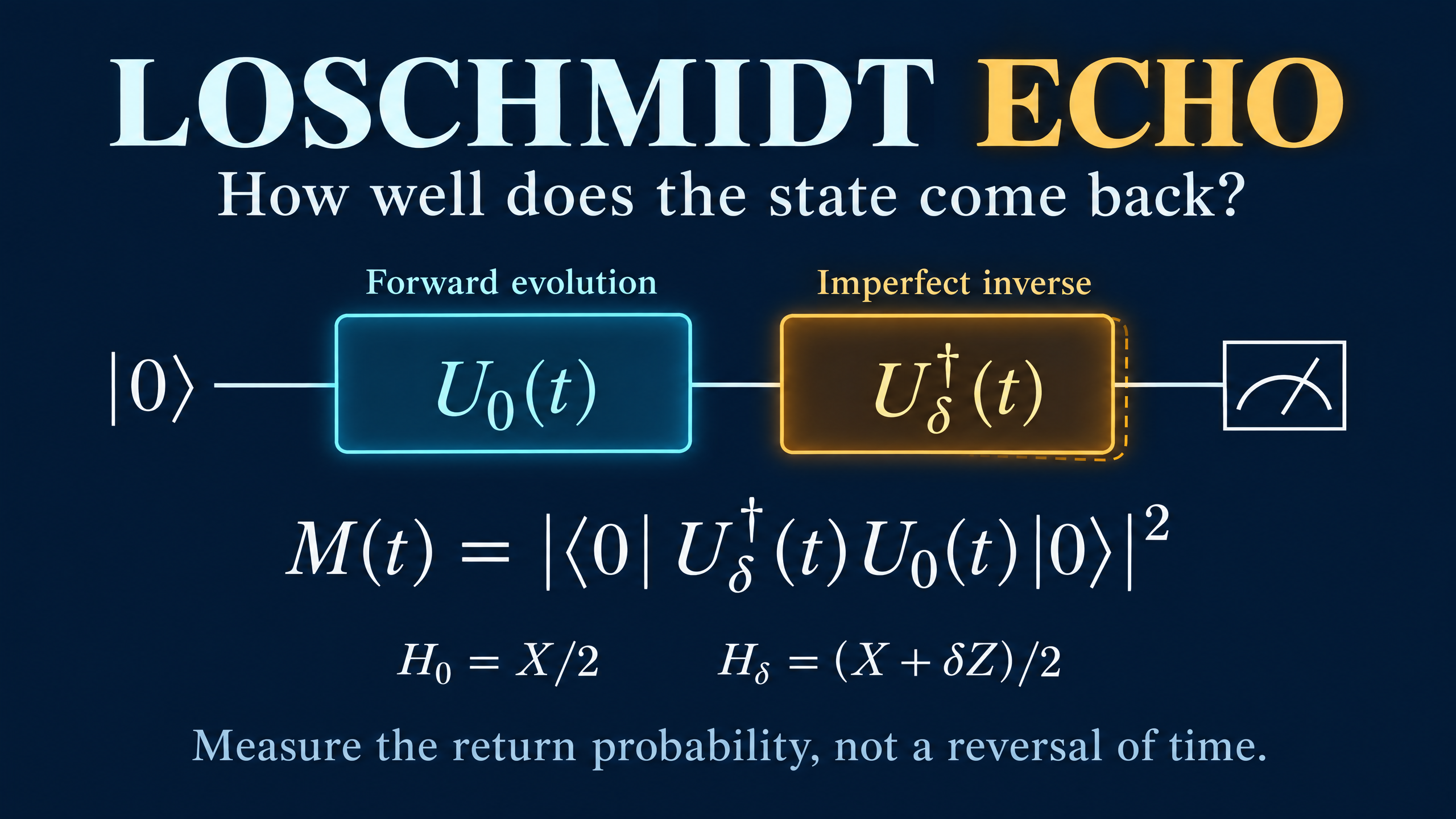
Loschmidt Echo: What an Imperfect Inverse Reveals
Run a quantum evolution forward, then try to undo it. A one-qubit simulation shows what the return probability reveals, and why a good echo is not proof of a perfect circuit.
A quantum gate is reversible in the mathematical sense: follow a unitary U with its exact inverse, and you get back the input state. Real experiments make that sentence less comfortable. What happens if the operation meant to undo the evolution is slightly wrong?
The Loschmidt echo turns that question into a measurable return probability. It is useful for studying how sensitive quantum dynamics are to a perturbation. It also offers a practical warning for programmers: a circuit that returns to its starting point has passed a consistency check, not necessarily a correctness test.
Let's build the smallest example that makes both ideas visible.
Forward evolution, then an imperfect inverse
Start with a normalized state |psi>. Set hbar = 1, so we can write the intended forward evolution as
U0(t) = exp(-i H0 t).
Suppose the inverse leg is instead implemented as
Udelta(t)† = exp(+i Hdelta t),
where Hdelta differs from H0. The final state is
|echo(t)> = Udelta(t)† U0(t)|psi>.
Here the dagger denotes the conjugate transpose. The sign in the exponential changes because we are attempting an inverse. Both legs still take place in ordinary forward laboratory time: the inverse leg corresponds to evolving under -Hdelta for duration t. The total duration of the two legs is 2t, not t.
The Loschmidt echo is the squared overlap with the initial state:
M(t) = |<psi|Udelta(t)† U0(t)|psi>|**2.
For Hdelta = H0, the two unitaries cancel and M(t) = 1. Otherwise, the return probability can fall below one. This is the standard definition used in the Loschmidt Echo review by Goussev and colleagues.
Why this is also a fidelity comparison
There is another way to read the same expression. Evolve two copies of the same initial state forward, one under H0 and one under Hdelta. Their squared overlap is
|<Udelta(t)psi|U0(t)psi>|**2 = M(t).
So the return experiment compares two evolutions without requiring us to prepare both output states and perform a separate overlap-test circuit. In this article, fidelity means this squared overlap of pure states. Other conventions use the square root of that squared overlap as the fidelity, so checking conventions matters.
For an initial |0>, M(t) is simply the probability of measuring 0 after the two legs. For a more general input prepared as A|0>, apply A† after the echo sequence, then measure 0. With ideal preparation and readout, that turns the same overlap into a computational-basis return probability.
A small tilt in the rotation axis
Use a single qubit with
H0 = X/2,
Hdelta = (X + delta*Z)/2.
X and Z are Pauli matrices. The intended evolution rotates around the Bloch sphere's X axis. The perturbed Hamiltonian adds a Z component, tilting the rotation axis and changing the rotation rate. The parameter delta is dimensionless in these chosen units; time is measured relative to the inverse scale of the X coefficient.
Prepare |0> and choose delta = 0.2. The forward leg uses H0, while the inverse leg uses -Hdelta. This mismatch is coherent: we have not introduced relaxation, random noise, or a measurement halfway through.
The thumbnail shows exactly this order: |0>, forward U0(t), imperfect inverse Udelta(t)†, then measurement. Remember that the rightmost matrix in the overlap formula acts first.
Test the echo in Python
This example needs NumPy and SciPy. Matrix exponentials are important here: exponentiating each matrix entry separately would not produce the intended unitary.
import numpy as np
from scipy.linalg import expm

X = np.array([[0, 1], [1, 0]], dtype=complex)
Z = np.array([[1, 0], [0, -1]], dtype=complex)
psi = np.array([1, 0], dtype=complex)
times = [0, 1, 2, 4, 6, 8]
delta = 0.2

print("t       M          norm       fidelity")
for t in times:
    U0 = expm(-1j * (X / 2) * t)
    Ud = expm(-1j * ((X + delta * Z) / 2) * t)
    echo = Ud.conj().T @ U0 @ psi
    M = abs(echo[0])**2
    fidelity = abs(np.vdot(Ud @ psi, U0 @ psi))**2
    norm = np.linalg.norm(echo)
    assert np.isclose(M, fidelity, atol=1e-12)
    assert np.isclose(norm, 1.0, atol=1e-12)
    print(f"{t:<7}{M:.6f}    {norm:.6f}    {fidelity:.6f}")

# Zero mismatch must recover the input at every tested time.
for t in times:
    U0 = expm(-1j * (X / 2) * t)
    echo0 = U0.conj().T @ U0 @ psi
    assert np.isclose(abs(echo0[0])**2, 1.0, atol=1e-12)
Expected output, rounded to six decimal places:
t       M          norm       fidelity
0      1.000000    1.000000    1.000000
1      0.997891    1.000000    0.997891
2      0.980113    1.000000    0.980113
4      0.972500    1.000000    0.972500
6      0.996279    1.000000    0.996279
8      0.980937    1.000000    0.980937
The norm column stays at one because the entire simulated process is unitary. A lower return probability does not mean the state has lost normalization. It means some amplitude ends up orthogonal to the starting state.
Notice the recovery near t = 6. This echo is not a steadily decaying curve. A finite, ideal one-qubit system can have coherent revivals. That is sensitivity to a mismatch, not evidence of irreversible decoherence or quantum chaos. The rich decay regimes studied in complex systems require much more than this minimal example.
The trap: a perfect echo can hide a wrong operation
Suppose a device implements some actual unitary V when you wanted U. If the second leg implements the exact actual inverse V†, then
V† V = I.
You get a perfect return even though the forward operation was wrong. Correlated calibration errors can therefore evade a round-trip test when their effects cancel between the legs. A test with only one initial state has an additional blind spot: an incorrect net operation can preserve that particular state while acting incorrectly on others.
A strong echo is useful evidence about a specific round trip and input. It is not, by itself, a certificate of the intended gate, an average gate fidelity, or a fault-tolerance benchmark. Varying input states, evolution times, and controlled perturbations makes the experiment more informative.
The code also assumes the inverse leg is a unitary generated by a known Hamiltonian. Real noisy hardware does not generally undo its noise when you reverse the gate sequence. An amplitude-damping event is not repaired by applying the inverse of the intended unitary.
How this relates to Hahn echo
The word echo connects several experiments. A Hahn echo uses a refocusing pulse to cancel certain phase accumulation, such as static detuning. It is historically connected to time-reversal ideas, but it does not generally invert every term in a system's Hamiltonian.
Here we explicitly compare a forward Hamiltonian with a perturbed inverse Hamiltonian. The focus is the return overlap and its sensitivity to the mismatch, rather than a specific refocusing-pulse sequence.
A useful next experiment
Change delta, repeat the calculation for |+>, and compare the two inputs. Then set Hdelta equal to H0 plus a multiple of the identity. That extra identity term produces only an overall phase in the return state, so M(t) stays one even though the returned state vector can have a different complex phase.
These checks capture the real lesson of the Loschmidt echo: it measures how well an evolution comes back for a chosen input, not whether every part of the journey was correct.