Pauli Measurement Grouping: Get More from the Same Shots
Group compatible Pauli terms, reuse bitstrings in Python, and see why commuting globally does not always mean sharing a local measurement basis.
A quantum energy calculation often looks simple on paper: write a Hamiltonian as a weighted sum of Pauli operators, estimate each expectation value, and add the results. On hardware, repeatedly preparing the state and collecting enough samples can dominate the work.
Measurement grouping asks a practical question: can the same batch of measurement outcomes tell us about several terms at once? For compatible terms, the answer is yes. The catch is that "commuting" has two meanings worth keeping separate when we choose a readout circuit.
One bitstring can supply several samples
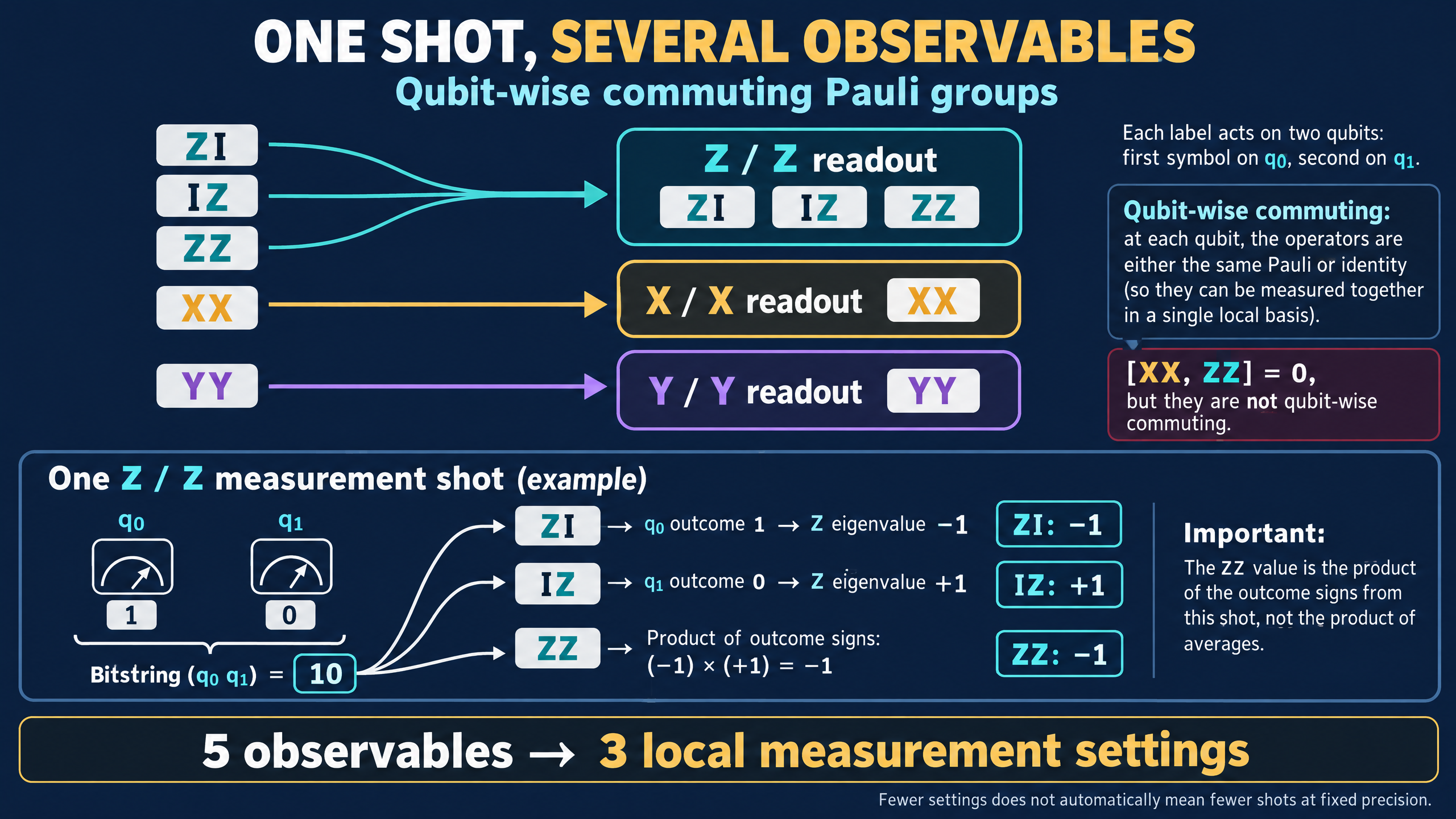
Consider two qubits measured in the computational, or Z, basis. A shot returns bits b0 and b1. Convert each bit to a Pauli eigenvalue: 0 becomes +1 and 1 becomes -1.
That single shot supplies three scores:
ZI: (-1)^b0
IZ: (-1)^b1
ZZ: (-1)^(b0+b1)
Here our strings run left to right as q0, q1. Thus ZI means Z on q0 and identity on q1. This is our explicit convention for the Python example, not Qiskit's displayed bit-order convention.
For the result 10, the three scores are -1, +1, and -1. Nothing has been cloned, and we have not learned a complete expectation value from one copy. We have obtained one sample for each compatible observable. Repeating the state preparation and measurement gives averages for all three from the same data.
Qiskit's observable-grouping documentation describes this idea using a general Pauli observable that specifies a shared readout basis, plus masks identifying which measured qubits contribute to each term.
The local compatibility rule
Two Pauli strings are qubit-wise commuting if, at every position, their letters match or at least one letter is I. This guarantees a common measurement basis built from single-qubit basis choices.
ZI, IZ, and ZZ pass that test. Their joint setting is simply Z readout on both qubits. The identity asks us to ignore a bit, not to perform another measurement.
For these five terms, a valid grouping is:
Z / Z setting: ZI, IZ, ZZ
X / X setting: XX
Y / Y setting: YY
To implement an X measurement using ordinary Z readout, apply H first. For Y, apply S† first, then H, then measure in Z. Z itself needs no basis rotation. Each setting starts with a fresh preparation of the same target state.
This reduces five separate term-by-term settings to three local settings. It does not mean that three shots are enough to estimate all five expectations accurately.
Commuting globally is a different test
XX and ZZ commute as two-qubit operators. On each qubit X and Z anticommute, but the two minus signs cancel in the tensor product.
They do not commute qubit-wise. A local measurement would need to choose both X and Z for the same qubit, which is not one product-basis setting.
There is no contradiction. Commuting operators share a simultaneous eigenbasis, but that basis need not be a product of single-qubit bases. For XX and ZZ, a Bell-basis measurement can reveal both eigenvalues, using an entangling basis-change circuit before readout. That is a different measurement strategy from the local grouping used here.
The GALIC study of Pauli grouping explains this distinction between fully commuting groups and the more restrictive qubit-wise commuting groups. The distinction matters because extra entangling gates can introduce circuit depth and noise.
Group the terms and reuse a histogram
This pure-Python example builds groups greedily. Then it reuses a hypothetical histogram of 100 Z-basis shots to estimate ZI, IZ, and ZZ. The histogram is illustrative data, not a device result or a full specification of the quantum state.
def qwc(a, b):
    if len(a) != len(b) or not set(a + b) <= set("IXYZ"):
        raise ValueError("Use equal-length Pauli strings")
    return all(x == y or x == "I" or y == "I"
               for x, y in zip(a, b))

def greedy_groups(words):
    groups = []
    for word in words:
        for group in groups:
            if all(qwc(word, other) for other in group):
                group.append(word)
                break
        else:
            groups.append([word])
    return groups

def z_score(word, bits):
    if (len(word) != len(bits) or not set(word) <= set("IZ")
            or not set(bits) <= set("01")):
        raise ValueError("Expected a Z-type word and matching bitstring")
    parity = sum(int(bit) for letter, bit in zip(word, bits)
                 if letter == "Z")
    return (-1) ** parity

words = ["ZI", "IZ", "ZZ", "XX", "YY"]
groups = greedy_groups(words)
print("Local-basis groups:", groups)

counts = {"00": 40, "01": 10, "10": 20, "11": 30}
shots = sum(counts.values())
for word in groups[0]:
    mean = sum(n * z_score(word, bits)
               for bits, n in counts.items()) / shots
    print(f"{word}: {mean:+.3f}")
Output:
Local-basis groups: [['ZI', 'IZ', 'ZZ'], ['XX'], ['YY']]
ZI: +0.000
IZ: +0.200
ZZ: +0.400
The ZZ mean is an average of the product of the two signs on each shot. It is not the product of the two separate averages. Here the latter would be 0 times 0.2, or zero, rather than 0.4. Keeping the shot-level correlations is essential.
This Z histogram does not provide the XX or YY means. Those require the corresponding additional settings. The greedy routine also makes no general claim to find the smallest possible grouping; its result can depend on the term order.
Fewer settings is not the whole cost calculation
For an energy estimate H = sum_j c_j P_j, compatible terms can share measurement data. That is the practical motivation behind grouping in variational algorithms, as illustrated in PennyLane's measurement-optimization tutorial.
Still, a fair comparison must target the same statistical precision. The coefficients, state-dependent variances, correlations between terms measured together, and allocation of shots between groups all matter. A smaller number of groups is not automatically a proportional reduction in the total number of shots.
On real hardware, compare the measurement circuits too. Larger groups that require entangling readout gates may trade fewer settings for more error. Local grouping offers a straightforward starting point: choose compatible bases, preserve the correlations in each bitstring, and extract every relevant observable from the data you already paid to collect.