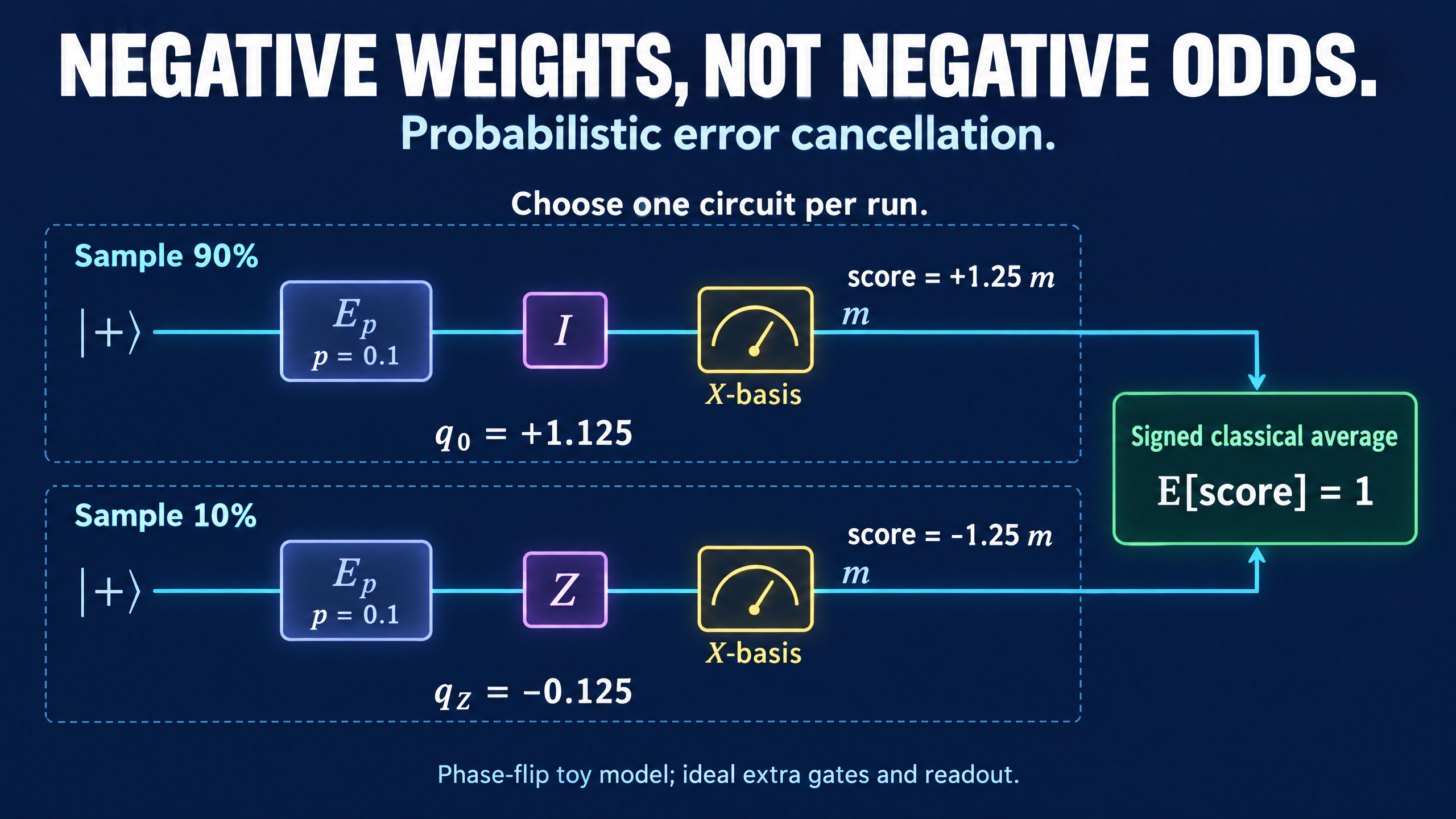
Probabilistic Error Cancellation: Negative Weights, Not Negative Odds
Negative PEC coefficients are not negative sampling probabilities. A tested one-qubit example shows how signed scores remove bias and increase uncertainty.
A noisy quantum circuit can give you a biased average even after millions of shots. More shots shrink the statistical error around the wrong value. Probabilistic error cancellation, or PEC, tackles that bias by combining results from different noisy circuit variants with signed weights.
The negative signs do not describe impossible experimental probabilities. They belong to the classical estimator. Every circuit is sampled with an ordinary, nonnegative probability, and no individual run is magically restored to a noise-free state.
A one-qubit phase-flip model makes the distinction concrete.
Two noisy variants can reproduce one ideal channel
Suppose the desired operation is an idle, but the qubit experiences a Z error with probability p:
E_p(rho) = (1-p) rho + p Z rho Z
Take 0 <= p < 1/2. The channel leaves the Z component of the Bloch vector unchanged and multiplies its X and Y components by lambda = 1-2p.
Assume we can run two variants:
F_0(rho) = E_p(rho)
F_Z(rho) = Z E_p(rho) Z
For this toy model, state preparation, the extra Z operation, and measurement are ideal. Only the specified phase-flip channel is noisy. Real PEC must characterize the operations it actually implements, including any additional relevant errors.
The identity channel can be written as
rho = q_0 F_0(rho) + q_Z F_Z(rho)

q_0 = (1-p)/(1-2p)
q_Z = -p/(1-2p)
You can verify the identity by expanding both variants into rho and Z rho Z. The unwanted coefficient cancels, leaving coefficient one on rho. Equivalently, q_0+q_Z = 1 preserves the unchanged Z component, while lambda(q_0-q_Z) = 1 restores the attenuated X and Y components.
This is a linear reconstruction of a channel, not a physical mixture with a negative probability. At p = 0.1, the coefficients are 1.125 and -0.125. Their sum is one, but one is negative and the other exceeds one. The original error-mitigation paper by Temme, Bravyi, and Gambetta develops this quasiprobability approach for ideal circuits represented using noisy implementations.
Turn those weights into an experiment
Define the coefficient norm
gamma = |q_0| + |q_Z|
Sample variant j with probability |q_j|/gamma. If a Pauli measurement returns m = +1 or -1, record the score
score = gamma sign(q_j) m
Its average over both the variant choice and the measurement outcome equals the ideal expectation value. The absolute values determine how often to run each variant; the signs determine how to score the result. This is the sampling rule described in the quasiprobability-method formulation.
For p = 0.1, gamma is 1.25. Run F_0 with probability 0.9 and F_Z with probability 0.1. Multiply an F_0 measurement by +1.25, or an F_Z measurement by -1.25. Average all the scores, keeping both kinds of runs.
This is not postselection. A negative-weight run is not a failed shot to discard.
Check the whole sampler in NumPy
Prepare |+> and measure X after the noisy idle. The ideal X expectation is one. Without mitigation, the phase flips reduce it to 0.8. Adding Z after the noise reverses that variant's X expectation to -0.8.
The code below enumerates the four possibilities: two circuit variants times two measurement outcomes. It calculates the estimator's exact mean and variance rather than printing a lucky finite-shot result.
import numpy as np

p = 0.1
Z = np.diag([1.0, -1.0])
X = np.array([[0.0, 1.0], [1.0, 0.0]])
plus = np.array([1.0, 1.0]) / np.sqrt(2)
rho = np.outer(plus, plus.conj())

noisy = (1 - p) * rho + p * Z @ rho @ Z
variants = [noisy, Z @ noisy @ Z]
q = np.array([(1 - p) / (1 - 2 * p), -p / (1 - 2 * p)])
gamma = np.abs(q).sum()
sampling = np.abs(q) / gamma
means = np.array([np.trace(X @ state).real for state in variants])

# Channel reconstruction is not itself a sampled physical state.
reconstructed = q[0] * variants[0] + q[1] * variants[1]
assert np.allclose(reconstructed, rho)

joint_probabilities, scores = [], []
for j in range(2):
    for outcome in [1, -1]:
        joint_probabilities.append(
            sampling[j] * (1 + outcome * means[j]) / 2
        )
        scores.append(gamma * np.sign(q[j]) * outcome)

probabilities = np.array(joint_probabilities)
scores = np.array(scores)
assert np.all(probabilities >= -1e-12)
assert np.isclose(probabilities.sum(), 1.0)
mean = np.dot(probabilities, scores)
variance = np.dot(probabilities, scores ** 2) - mean ** 2

print(f"Noisy X mean: {means[0]:.6f}")
print("Coefficients:", q)
print("Sampling probabilities:", sampling)
print(f"Signed estimator mean: {mean:.6f}")
print(f"Single-shot variance: {variance:.6f}")
print(f"Standard error at 10000 shots: {np.sqrt(variance / 10000):.6f}")
print(f"Gamma squared: {gamma ** 2:.6f}")
Output:
Noisy X mean: 0.800000
Coefficients: [ 1.125 -0.125]
Sampling probabilities: [0.9 0.1]
Signed estimator mean: 1.000000
Single-shot variance: 0.562500
Standard error at 10000 shots: 0.007500
Gamma squared: 1.562500
These are exact calculations for the stated noise model, not hardware data. The standard error assumes independent shots and the exact coefficients. It does not include calibration uncertainty or model error.
For this particular final X measurement, the random Z operation can be absorbed into outcome relabeling. The estimator then reduces to dividing the unmitigated X average by 1-2p. The explicit two-variant sampler is useful here because it exposes the machinery of PEC, not because this simplest case needs extra physical gates.
Bias cancellation comes with a variance bill
Each signed Pauli score has magnitude gamma. If its ideal mean is mu, its variance is gamma^2-mu^2, bounded by gamma^2. Thus gamma^2 controls a standard worst-case sampling-cost bound. It is not a universal ratio between the exact variances of every ideal and mitigated experiment. In our example, ideal X measurement on |+> is deterministic, while the mitigated estimator still fluctuates.
A finite sample average can even lie outside the physical expectation range [-1, 1]. The estimator is not a density matrix, and an out-of-range estimate does not imply that the hardware produced an impossible state. Automatically clipping it would generally introduce bias.
For a straightforward gate-by-gate decomposition, the coefficient norms multiply across corrected locations. The corresponding worst-case sampling bound can therefore grow exponentially with the amount of noise being canceled. IBM's PEC tutorial explains this overhead and why identifying errors irrelevant to a target observable can reduce the cost.
The model is just as important as the shot budget. If the true phase-flip probability is p_actual but the final-X rescaling uses p_model, the corrected mean for this example is
(1 - 2 p_actual) / (1 - 2 p_model)
More shots converge toward that value, not necessarily toward one. At p = 1/2, the channel has erased all X and Y information, so this inverse does not exist. As p approaches that point, the coefficients and sampling cost diverge.
PEC is therefore a method for reconstructing selected ideal statistics under a trusted operational model. It is not a way to make each noisy qubit clean again. The practical question is whether the bias you remove is worth the statistical uncertainty and calibration work you add.