Quantum Amplitude Estimation: Read a Probability from Two Phase Peaks
Use a tested NumPy example to see why two phase-estimation peaks can encode one success probability, and why more precision costs coherent circuit work.
Suppose a quantum program raises a success flag with probability a. You could run it repeatedly, count the successes, and estimate a from their frequency. Quantum amplitude estimation takes a different route: it builds a rotation whose eigenphases encode that probability, then estimates those phases.
The surprising part is that two different phase-estimation outcomes can represent exactly the same answer. Understanding that pair makes the algorithm much less mysterious, and helps explain why extra counting qubits are not free precision.
Start with a coherent experiment
Let A be a unitary state-preparation circuit. Split its output into normalized, orthogonal bad and good components:
|psi> = A|0> = sqrt(1-a)|bad> + sqrt(a)|good>
a = sin^2(theta), with 0 < theta < pi/2
Here a is a probability; the good component's amplitude is sqrt(a). The good subspace might be defined by a flag qubit being one. We exclude the deterministic endpoints in this explanation so both components are present.
Amplitude estimation assumes more than access to a stream of measured successes and failures. You need coherent access to the preparation and its inverse, plus a way to mark good states. For the original phase-estimation construction, you also need controlled powers of the resulting Grover operator.
Two reflections make the hidden rotation
Use a good-state phase flip and a reflection about the prepared state:
S_good = I - 2 Pi_good
R_psi  = 2|psi><psi| - I
Q      = R_psi S_good
Pi_good projects onto the good subspace. In the two-dimensional span of |bad> and |good>, Q has the matrix
       [ cos(2 theta)  -sin(2 theta) ]
Q  =   [ sin(2 theta)   cos(2 theta) ]
Its eigenvalues are exp(+2i theta) and exp(-2i theta). This is the key bridge: the unknown probability a determines an angle, and that angle appears as a unitary eigenphase. The original amplitude amplification and estimation paper develops this connection.
The reflection is implementable as A R_0 A-dagger, where R_0 = 2|0><0| - I. Some references instead define the zero-state phase flip with the opposite sign and put an explicit minus sign in Q. These descriptions agree when their conventions are used consistently. Do not casually drop the sign of Q in a controlled circuit: what would be a global phase on the target alone becomes a relative phase on the control.
Why the readout has two peaks
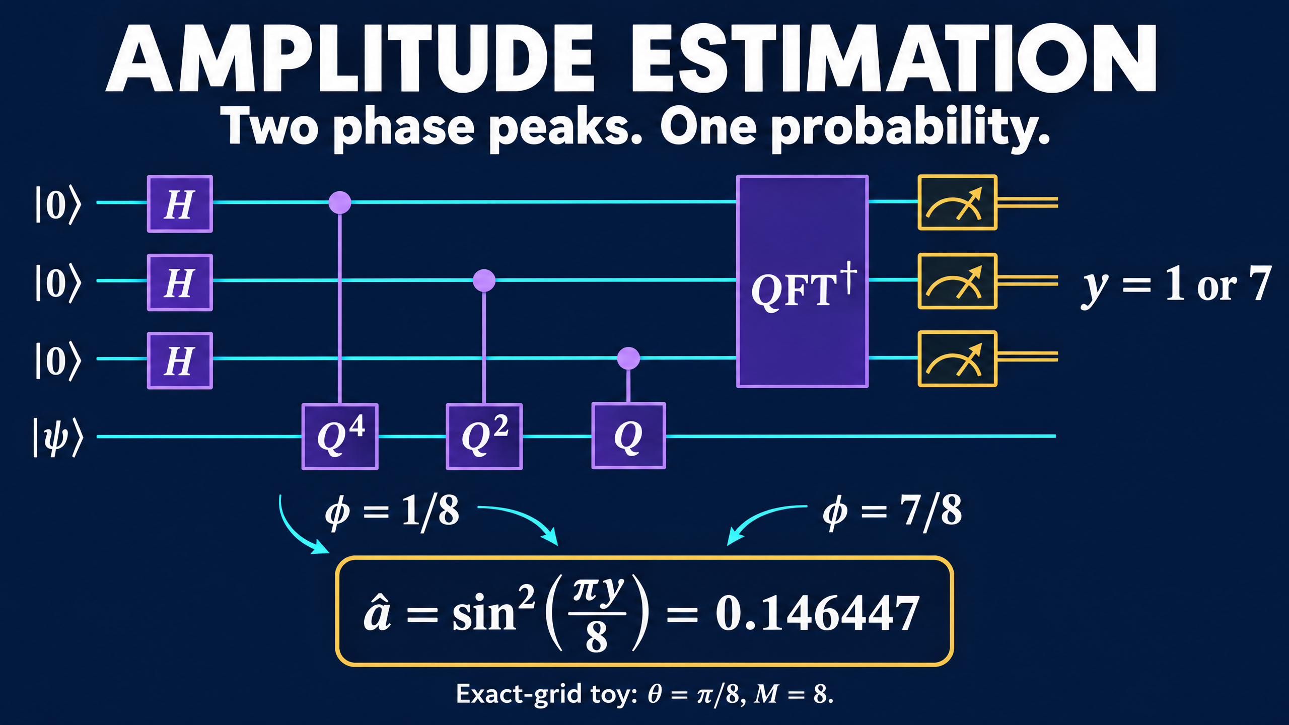
Phase estimation describes an eigenvalue as exp(2 pi i phi), with phi interpreted modulo one. The two eigenphases above correspond to
phi_plus  = theta / pi
phi_minus = 1 - theta / pi
The input |psi> is a superposition of the two eigenvectors, not generally one eigenvector. The counting register therefore has contributions from both phases.
With m counting qubits, let M = 2^m. Measuring the counting register gives an integer y from zero to M-1. Decode it as
a_hat = sin^2(pi y / M)
Values y and M-y give the same decoded probability. The mirrored peaks are not two conflicting answers.
For a clean example, choose theta = pi/8 and m = 3. Then M = 8, the eigenphases are 1/8 and 7/8, and ideal phase estimation returns y = 1 or y = 7, each with probability one half. Both decode to sin^2(pi/8), about 0.146447.
Simulate the complete counting distribution
The example below uses one data qubit, with |1> marked good, and three counting qubits. A is a real Y rotation that prepares the desired test probability. We supply a explicitly to construct a known test instance; this is not a claim that estimating an already supplied number is useful.
The array before the Fourier transform represents the joint state after a uniform counting superposition and controlled powers of Q. Its row k is Q^k|psi>/sqrt(M). NumPy's normalized FFT supplies the inverse Fourier transform with negative exponent, acting on the counting index. Summing over the remaining data index gives the counting probabilities.
import numpy as np


def counting_distribution(a, m):
    M = 2 ** m
    c, s = np.sqrt(1 - a), np.sqrt(a)
    A = np.array([[c, -s], [s, c]])
    psi = A @ np.array([1.0, 0.0])
    Z = np.diag([1.0, -1.0])

    # Z is R_0 here, and also flips the good state |1>.
    Q = A @ Z @ A.conj().T @ Z
    assert np.allclose(Q.conj().T @ Q, np.eye(2))

    joint = np.array([
        np.linalg.matrix_power(Q, k) @ psi
        for k in range(M)
    ]) / np.sqrt(M)
    after_iqft = np.fft.fft(joint, axis=0, norm="ortho")
    probabilities = np.sum(abs(after_iqft) ** 2, axis=1)
    decoded = np.sin(np.pi * np.arange(M) / M) ** 2
    assert np.isclose(probabilities.sum(), 1.0)
    return probabilities, decoded


probs, estimates = counting_distribution(np.sin(np.pi / 8) ** 2, 3)
for y in np.flatnonzero(probs > 1e-10):
    print(f"y={y}: P={probs[y]:.6f}, a_hat={estimates[y]:.6f}")

probs_off, estimates_off = counting_distribution(0.2, 3)
modal_estimate = estimates_off[np.argmax(probs_off)]
print(f"Off-grid modal estimate: {modal_estimate:.6f}")
Output:
y=1: P=0.500000, a_hat=0.146447
y=7: P=0.500000, a_hat=0.146447
Off-grid modal estimate: 0.146447
These are exact ideal-state probabilities, not sampled shot counts or hardware results. The code constructs a small joint state directly; it is not a gate compiler or a resource estimate.
The second case matters. When a = 0.2, the eigenphases do not land exactly on the three-bit phase grid. The most likely decoded value is still about 0.146447, and other outcomes have nonzero probability. A modal estimate describes the distribution's highest peak, not a promise about every shot. The canonical single-readout decoder has finite resolution, and its probability grid is not uniformly spaced.
Count coherent work, not just qubits
For fixed confidence and worst-case additive error epsilon, independent Bernoulli sampling needs on the order of 1/epsilon^2 samples. Ideal amplitude estimation can achieve that accuracy with on the order of 1/epsilon coherent oracle uses. This is a query-complexity comparison under the required access assumptions, not a guaranteed wall-clock speedup.
The canonical circuit uses controlled Q, Q^2, Q^4, and so on. With m counting qubits, implementing those powers by repetition costs a total of M-1 uses of Q in that stage. Adding one counting qubit doubles M. A diagram with one box labeled Q^128 has not made 128 applications disappear.
State preparation, reversing A, the good-state test, control overhead, and coherent circuit depth all matter. Noise can erase the benefit before the asymptotic query advantage becomes useful. Research on low-depth amplitude estimation studies explicit tradeoffs between sequential depth and total oracle calls.
Other amplitude-estimation families avoid the large inverse-QFT counting register and infer the angle from measurements at selected Grover powers. They change the circuit and inference strategy; they do not turn long coherent evolutions or repeated experiments into free resources.
The useful idea to keep is simple: amplitude estimation measures a probability indirectly through a rotation angle. Two mirrored phase peaks can encode one probability, while the cost of resolving that angle is paid in coherent work, not merely in the number of bits printed at the end.