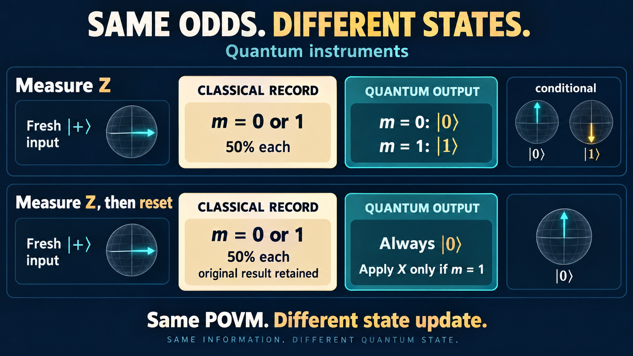
Quantum Instruments: Same Measurement Odds, Different States
Identical measurement counts do not imply identical quantum outputs. Compare a projective measurement with measurement plus reset, and test their different second measurements in NumPy.
Two quantum programs produce the same measurement histogram. Do they perform the same measurement?
If the qubit is thrown away immediately afterward, the histogram may be all you need. If the program keeps using that qubit, it is not enough. Two devices can report exactly the same outcome probabilities for every input and still leave different quantum states behind.
The distinction has a name: a POVM describes the measurement odds, while a quantum instrument also describes what happens to the quantum output. A one-qubit example makes the difference surprisingly concrete.
Separate the classical record from the quantum output
Suppose we measure a qubit in the computational basis. Write the two projectors as
P0 = |0><0| and P1 = |1><1|.
For a density matrix rho, outcome m occurs with probability
p(m) = Tr(Pm rho).
The positive operators P0 and P1 sum to the identity. Together they form a positive operator-valued measure, or POVM. A projective measurement is a special case of a POVM; the phrase does not require nonorthogonal effects or extra outcomes.
IBM's general-measurement lesson develops this probability rule. Those effects tell us which classical results to expect. They do not, by themselves, specify the state of a retained measured qubit.
For that, we need a state-update rule as well.
Two implementations with identical odds
Our first implementation is the ideal projective state update, sometimes called the Lüders instrument. It uses one Kraus operator per outcome:
K0 = P0, K1 = P1.
The unnormalized quantum state in branch m is Km rho Km†. Its trace is the probability of that branch. When the trace is nonzero, divide by it to obtain the conditional density matrix. In this particular measurement, outcome 0 leaves |0> and outcome 1 leaves |1>.
Now change the program. Perform the same ideal Z measurement, retain its classical result m, and apply X to the qubit only when m = 1. This is a measurement followed by conditional feedback, with operators
L0 = |0><0|, L1 = |0><1|.
The second operator is X P1: the outcome-1 branch first projects onto |1>, then flips that state to |0>.
Check the effects:
K0† K0 = L0† L0 = P0
and
K1† K1 = L1† L1 = P1.
Since outcome probabilities depend on these effects, both implementations have the same first measurement statistics for every input rho, not just for a carefully chosen test state. Yet the feedback implementation leaves the qubit in |0> in either branch.
Crucially, it does not rewrite the recorded result. The classical bit can still say 1 while the output qubit is |0>. Resetting the qubit and changing the measurement record are different operations.
What an instrument adds
More generally, an instrument assigns a completely positive, trace-nonincreasing map to each classical outcome m. In finite dimensions we can write each branch as
I_m(rho) = sum_a K_(m,a) rho K_(m,a)†.
Its associated POVM effect is
E_m = sum_a K_(m,a)† K_(m,a).
Then p(m) = Tr(I_m(rho)) = Tr(E_m rho). Summing all branch maps gives a trace-preserving quantum channel. If we keep the classical record too, the combined output is a classical-quantum state, with each outcome paired with its corresponding unnormalized quantum branch.
Our example needs only one Kraus operator for each outcome. A general instrument can require several per outcome, so a single operator is not the full definition.
The formal distinction and examples of different instruments sharing a POVM are developed in Leppäjärvi and Sedlák's paper on quantum instruments. The important programming question is simple: does your measurement specification describe only the reported bit, or also the state you plan to use next?
Test the difference with a second measurement
Start with |+>, so both first outcomes have probability 1/2. After an ordinary ideal Z measurement, forgetting the result gives the qubit state I/2. After measurement plus feedback, forgetting the result gives |0><0|.
A second Z measurement separates them. The ordinary projective measurement is repeatable in this ideal setup: the second result equals the first. In the feedback version, the second result is always 0. It disagrees with the first result on the half of runs where the first result was 1.
The following NumPy calculation keeps the first outcome branches separate. It computes joint probabilities exactly, without random sampling or a hardware backend.
import numpy as np

zero = np.array([1, 0], dtype=complex)
one = np.array([0, 1], dtype=complex)
P0 = np.outer(zero, zero.conj())
P1 = np.outer(one, one.conj())
plus = (zero + one) / np.sqrt(2)
rho = np.outer(plus, plus.conj())

instruments = {
    "measure": [P0, P1],
    "measure + reset": [P0, np.outer(zero, one.conj())],
}

for name, operators in instruments.items():
    effects = [K.conj().T @ K for K in operators]
    assert np.allclose(effects[0], P0)
    assert np.allclose(effects[1], P1)
    assert np.allclose(sum(effects), np.eye(2))

    branches = [K @ rho @ K.conj().T for K in operators]
    first = np.array([np.trace(b).real for b in branches])
    output = sum(branches)

    # Rows: first result m. Columns: second Z result n.
    joint = np.array([
        [np.trace(P @ branch).real for P in [P0, P1]]
        for branch in branches
    ])
    assert np.allclose(joint.sum(axis=1), first)
    second_one = joint[:, 1].sum()
    disagreement = joint[0, 1] + joint[1, 0]

    print(name)
    print("  first probabilities:", np.round(first, 3))
    print("  output diagonal:", np.round(np.diag(output).real, 3))
    print(f"  P(second=1): {second_one:.3f}")
    print(f"  P(second != first): {disagreement:.3f}")
The output is
measure
  first probabilities: [0.5 0.5]
  output diagonal: [0.5 0.5]
  P(second=1): 0.500
  P(second != first): 0.000
measure + reset
  first probabilities: [0.5 0.5]
  output diagonal: [1. 0.]
  P(second=1): 0.000
  P(second != first): 0.500
The first histograms match. The joint records do not. Looking only at the first classical output would miss the entire difference.
The lesson for dynamic circuits
When a circuit ends at measurement, an outcome-only model can be perfectly appropriate. When a circuit continues with feedback, qubit reuse, or another measurement, the state update becomes part of the program's behavior.
That does not mean real hardware always follows the ideal projective or perfect-reset models above. Readout errors, imperfect feedback, and other dynamics can change both the observed statistics and the remaining state. These examples specify ideal operations so that the distinction is visible without those complications.
Nor does a reset recover the unknown input. It deliberately prepares a fixed state. Both implementations destroy the input's Z-basis coherence in this example; the feedback version additionally makes the retained qubit independent of the recorded outcome.
So when two measurement implementations agree on their counts, ask one more question before treating them as interchangeable: what quantum state comes out, and will the rest of the program notice?