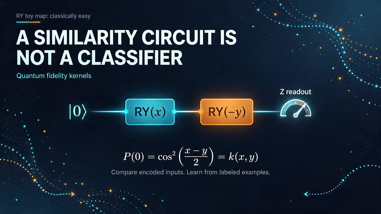
Quantum Kernels: A Similarity Circuit Is Not a Classifier
Build a one-qubit fidelity kernel, prove its matrix is positive semidefinite, and use it in a tiny classical learner without mistaking similarity for a class label.
A quantum circuit can compare two data points without deciding which class either point belongs to. That distinction is easy to miss when a machine-learning demo ends with an accuracy score.
In a fidelity-kernel workflow, the quantum part estimates similarities. A classical learning algorithm uses those similarities, together with training labels, to make predictions. Let's build a tiny example where the circuit, the kernel matrix, and the learning step are all visible. The example is deliberately easy to simulate, so it explains the mechanism without suggesting a quantum speedup.
Turn data into states, then compare them
Choose a data-dependent unitary U(x) and prepare a normalized feature state:
|phi(x)> = U(x)|0...0>
k(x,y) = |<phi(y)|phi(x)>|^2
This article uses the squared-overlap convention. For pure feature states, it is also their squared fidelity. Other quantum kernels use other constructions, so this is a particular useful family, not the definition of every quantum kernel.
To estimate this entry, start in the all-zero state, apply U(x), then apply U(y)-dagger, and measure every qubit in the computational basis. The probability of the all-zero outcome is exactly k(x,y) in the ideal circuit.
Notice the order: the inverse of y's feature circuit comes after x's circuit. Measuring just one selected qubit is generally not enough. IBM's quantum-kernel lesson develops this compute-and-uncompute construction. The Qiskit Machine Learning tutorial shows how the resulting matrix connects to classical learning tools.
There is no class label in this probability. An entry near one says that these encoded states are similar. Whether that similarity helps separate the desired labels depends on the feature map and dataset.
A one-qubit example you can solve exactly
Use one real input angle x, in radians, and set U(x) = RY(x), with
RY(x) = [[cos(x/2), -sin(x/2)],
         [sin(x/2),  cos(x/2)]]
The overlap circuit is simply RY(x) followed by RY(-y). Its all-zero probability is
k(x,y) = cos^2((x-y)/2)
       = (1 + cos(x-y))/2
Equal angles have similarity one. Angles separated by pi have similarity zero. Angles separated by 2 pi represent the same physical feature state up to a global phase, so they again have similarity one. This encoding treats the input as periodic. It would be a poor default for a quantity whose two endpoints must remain distinct.
Why the ideal kernel matrix is positive semidefinite
For training points x_1 through x_m, form K[i,j] = k(x_i,x_j). In the noiseless pure-state construction, K is symmetric, has ones on its diagonal, and is positive semidefinite, or PSD.
The last property is more than an aesthetic preference. Define the density-operator feature rho_x = |phi(x)><phi(x)|. Then
k(x,y) = Tr(rho_x rho_y)
For real coefficients c_i, the quadratic form c-transpose K c is Tr(A^2), where A = sum_i c_i rho_i is Hermitian. That is nonnegative. So the squared-overlap kernel is a Gram matrix in operator space, even though taking entrywise squares of an arbitrary matrix would not generally preserve all the properties you want.
Our toy example has an even simpler classical feature vector:
f(x) = [1, cos(x), sin(x)] / sqrt(2)
k(x,y) = dot(f(x), f(y))
This also proves PSD and bounds the matrix rank by three, regardless of the number of training points. A one-qubit encoding does not automatically produce a classically difficult kernel. Here its entire geometry fits in three ordinary real features.
Build the matrix and use it
The code needs only NumPy. It computes each entry from the actual rotation matrices, checks the closed form and classical feature map, then fits a regularized kernel-ridge model to four labeled points. Predicting the sign of its score gives a simple binary decision rule.
import numpy as np


def ry(angle):
    c, s = np.cos(angle / 2), np.sin(angle / 2)
    return np.array([[c, -s], [s, c]])


def kernel(x, y):
    zero = np.array([1.0, 0.0])
    output = ry(y).conj().T @ ry(x) @ zero
    return float(abs(output[0]) ** 2)


train = np.array([0, np.pi / 2, np.pi, 3 * np.pi / 2])
labels = np.array([1.0, 1.0, -1.0, -1.0])
K = np.array([[kernel(x, y) for y in train] for x in train])
closed = (1 + np.cos(train[:, None] - train[None, :])) / 2
features = np.column_stack((np.ones(4), np.cos(train),
                            np.sin(train))) / np.sqrt(2)
assert np.allclose(K, closed)
assert np.allclose(K, features @ features.T)
assert np.allclose(np.diag(K), 1)
eigenvalues = np.linalg.eigvalsh(K)
assert eigenvalues.min() >= -1e-12

regularization = 0.1
alpha = np.linalg.solve(K + regularization * np.eye(4), labels)
test = np.array([np.pi / 4, 5 * np.pi / 4])
K_test = np.array([[kernel(x, y) for y in train] for x in test])
scores = K_test @ alpha
predictions = np.where(scores >= 0, 1, -1)

np.set_printoptions(precision=6, suppress=True)
print("kernel matrix:")
print(np.round(K, 6))
print("eigenvalues:", np.round(np.maximum(eigenvalues, 0), 6))
print("predicted labels:", predictions)
Output:
kernel matrix:
[[1.  0.5 0.  0.5]
 [0.5 1.  0.5 0. ]
 [0.  0.5 1.  0.5]
 [0.5 0.  0.5 1. ]]
eigenvalues: [0. 1. 1. 2.]
predicted labels: [ 1 -1]
The tiny negative eigenvalue that floating-point arithmetic may produce is checked against a tolerance before being clipped for display. That display cleanup is not a general repair procedure for an experimentally estimated kernel.
The learner uses the labels through alpha = (K + lambda I)^(-1) labels. The code solves the linear system rather than explicitly inverting its matrix. Lambda here is the positive regularization value in this stated convention. Different libraries may scale regularization differently. The two test predictions illustrate the pipeline, not a meaningful generalization benchmark. The ridge scores themselves are not probabilities.
Where the real costs hide
On hardware, each ideal kernel entry becomes an estimate from repeated shots. With S shots and an ideal success probability k, the standard deviation of the all-zero frequency is sqrt(k(1-k)/S). Circuit errors add bias that this binomial expression does not describe.
For m training points, exploiting the ideal symmetry leaves m(m-1)/2 distinct off-diagonal entries. Each still needs sampling effort; comparing new points to the training set requires more entries. The ideal diagonal is known, but a noisy compute-and-uncompute experiment need not return to zero with probability one.
Finite-shot estimates, hardware errors, or direction-dependent implementations can yield a matrix that is asymmetric or has negative eigenvalues. Symmetrizing or projecting onto the PSD cone can make it suitable for particular downstream methods, but changes the estimate. It is not evidence that the original experimental matrix was an exact fidelity kernel.
Finally, a feature space with many dimensions is not a guarantee of better predictions or lower total cost. You still need a useful encoding, an accuracy budget, classical baselines, and a learning task for which the resulting similarities matter. For our RY example, the explicit three-feature formula is already an efficient classical baseline.
The quantum circuit supplies a similarity rule. The feature map determines its geometry, and the learner turns that geometry plus labeled examples into a prediction. Keeping those jobs separate makes quantum-kernel demos easier to understand and much harder to oversell.