Quantum Memory Effects: When Lost Distinguishability Comes Back
Use a two-qubit NumPy model to see lost distinguishability return, understand information backflow, and learn what a trace-distance revival does and does not prove.
Two different qubit states can become indistinguishable if we look only at the qubit. Surprisingly, they can become distinguishable again later without an echo pulse or an error-correction procedure.
The missing ingredient is the environment. If it remains coupled to the qubit instead of being continually replaced by a fresh bath, correlations can carry a memory of the earlier state. A two-qubit model makes this effect visible with a short NumPy calculation.
Ask a question about two preparations
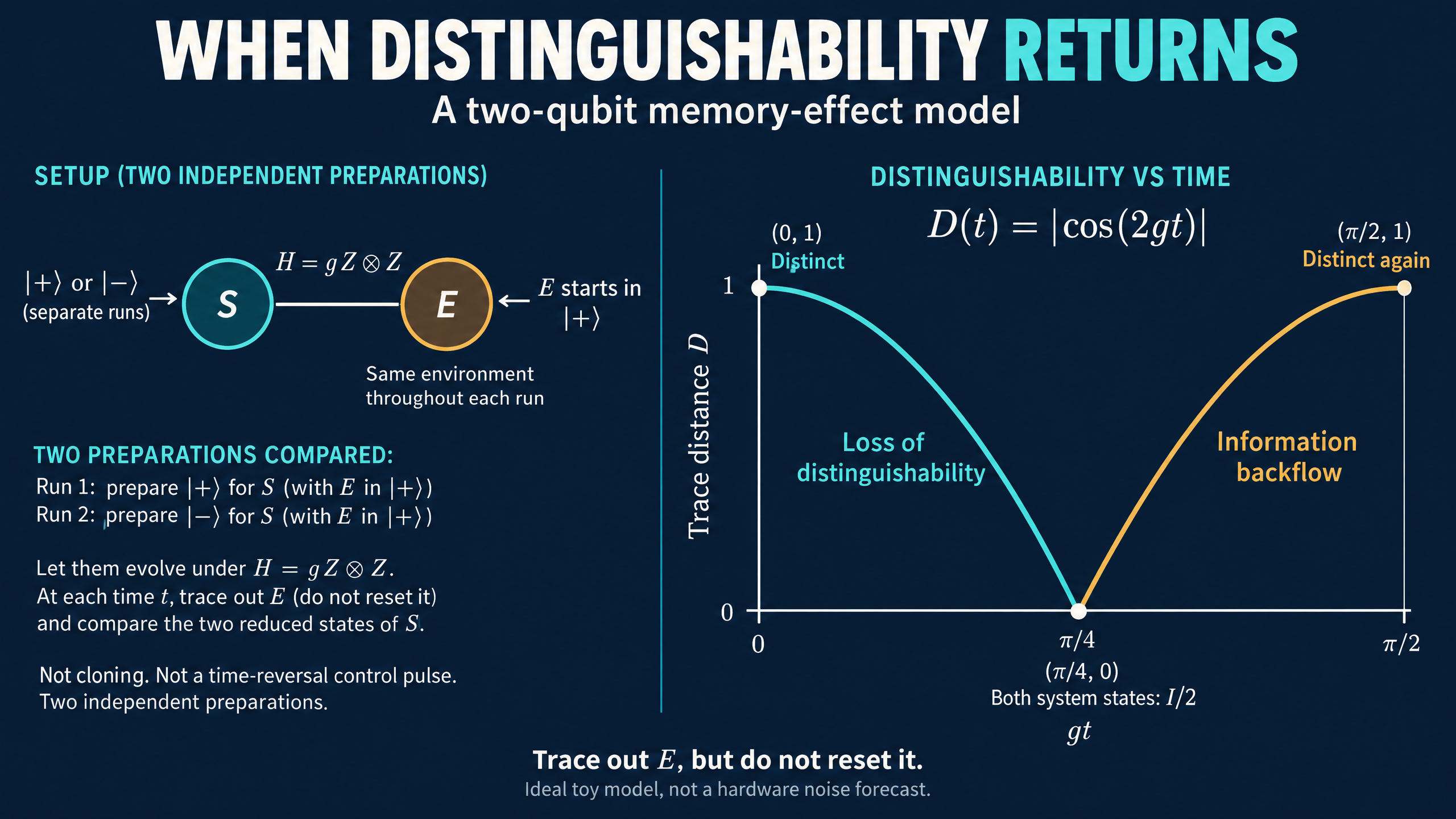
Prepare the system qubit in either |+> or |-> in separate runs. These orthogonal states can initially be distinguished perfectly.
To track what happens, use trace distance:
D(rho_a, rho_b) = (1/2) ||rho_a - rho_b||_1
For density matrices, D ranges from zero to one. Zero means the two states are identical; one means they are perfectly distinguishable. With equal prior probabilities, the best possible single-shot guessing probability is (1 + D)/2.
A physical quantum channel cannot increase trace distance when the same channel is applied to both states. If every later stage could be represented by a fresh channel acting only on the current system state, distinguishability could only stay constant or decrease.
A revival is therefore a useful witness of memory effects. This trace-distance approach is explained in the open-quantum-systems tutorial on information backflow.
Give the qubit a small environment
Let S be the system and E a second qubit. Set hbar = 1 and use the interaction Hamiltonian:
H = g Z_S tensor Z_E
U(t) = exp(-i H t)
Here g is a positive coupling frequency. The environment starts in |+>, with the same preparation in each independent run. Within a run, the same environment remains part of the joint evolution. We trace it out mathematically to evaluate the system state; we do not physically reset it at each time.
For system inputs |+> and |->, the reduced states are:
rho_plus(t)  = (1/2) [[1,  c(t)], [ c(t), 1]]
rho_minus(t) = (1/2) [[1, -c(t)], [-c(t), 1]]
c(t) = cos(2gt)
The populations do not change. Only the off-diagonal elements change, so this is a dephasing model rather than energy relaxation.
The trace distance follows directly:
D(t) = |cos(2gt)|
At gt = pi/4, both reduced states are I/2. Looking only at S gives no clue about which preparation was used. At gt = pi/2, the system states are distinct again: |+> has become |-> and |-> has become |+>.
The labels have swapped, but perfect distinguishability has returned.
Simulate the whole pair, then trace out E
The tensor-product ordering below is S first, E second. The partial trace sums over equal environment indices in the row and column of the joint density matrix.
import numpy as np

plus = np.array([1, 1], dtype=complex) / np.sqrt(2)
minus = np.array([1, -1], dtype=complex) / np.sqrt(2)
env = np.outer(plus, plus.conj())
g = 1.0

def system_state(ket, t):
    zz_diagonal = np.array([1, -1, -1, 1])
    U = np.diag(np.exp(-1j * g * t * zz_diagonal))
    rho = np.outer(ket, ket.conj())
    joint = U @ np.kron(rho, env) @ U.conj().T
    # Axes are S_row, E_row, S_column, E_column.
    return np.einsum('aibi->ab', joint.reshape(2, 2, 2, 2))

def trace_distance(a, b):
    # a-b is Hermitian, so its singular values are |eigenvalues|.
    return 0.5 * np.abs(np.linalg.eigvalsh(a - b)).sum()

print("gt/pi  trace distance")
for gt in np.linspace(0, np.pi / 2, 5):
    t = gt / g
    a = system_state(plus, t)
    b = system_state(minus, t)
    distance = trace_distance(a, b)
    print(f"{gt/np.pi:5.3f}  {distance:.6f}")
    assert np.isclose(distance, abs(np.cos(2 * gt)))
Output:
gt/pi  trace distance
0.000  1.000000
0.125  0.707107
0.250  0.000000
0.375  0.707107
0.500  1.000000
Each row is a separate evaluation of the joint evolution from the same initial product preparation. We are not measuring the system repeatedly during a single trajectory. Such measurements would change the dynamics.
Why this does not break channel contractivity
The evolution from the initial system state to any fixed later time is still a valid quantum channel: append the same environment state, evolve unitarily, and trace out E. The distance never exceeds its initial value of one.
What fails is the idea that there must also be a common system-only channel connecting every pair of intermediate times.
At gt = pi/4, our two system states are identical. No single channel acting only on that identical input could later produce two different outputs. Yet the full S-plus-E states are not identical. The joint state, including its correlations, retains information that the reduced system state alone does not contain.
Continued interaction makes some of that information accessible in S again. Calling this information backflow is an operational statement about the revival of distinguishability, not a claim that a message travels backward in time.
A witness, not a universal memory detector
For comparison, a simple memoryless dephasing model can have a coherence factor exp(-kappa t), with kappa positive. Its |+> versus |-> trace distance decays monotonically.
Even our two-qubit interaction behaves differently if we replace the environment with a fresh |+> qubit after every equal time step dt. Then each step multiplies this pair's distinguishability by |cos(2g dt)|. After n steps, the distance is |cos(2g dt)| to the power n, which cannot revive.
Trace-distance revivals witness failure of completely positive divisibility: the evolution cannot be broken into physical system-only channels between all intermediate times. The converse is not generally true. Some dynamics fail that divisibility test without showing a revival for any pair of system states. The comparative study of non-Markovianity measures explains why different definitions of quantum memory effects need not agree.
This example is an exact, ideal model with one environment qubit. It is not an experimental noise forecast, a model of every device, or evidence that memory effects are always beneficial. Its lesson is narrower and useful: once the environment retains a record of the past, the current state of the system need not be enough to predict what comes next.