Quantum Switch: Detect Anticommutation with Coherent Gate Order
Put two gate orders in a coherent superposition and a relative sign becomes a control-qubit readout. A NumPy example tests commuting, anticommuting, and intermediate cases.
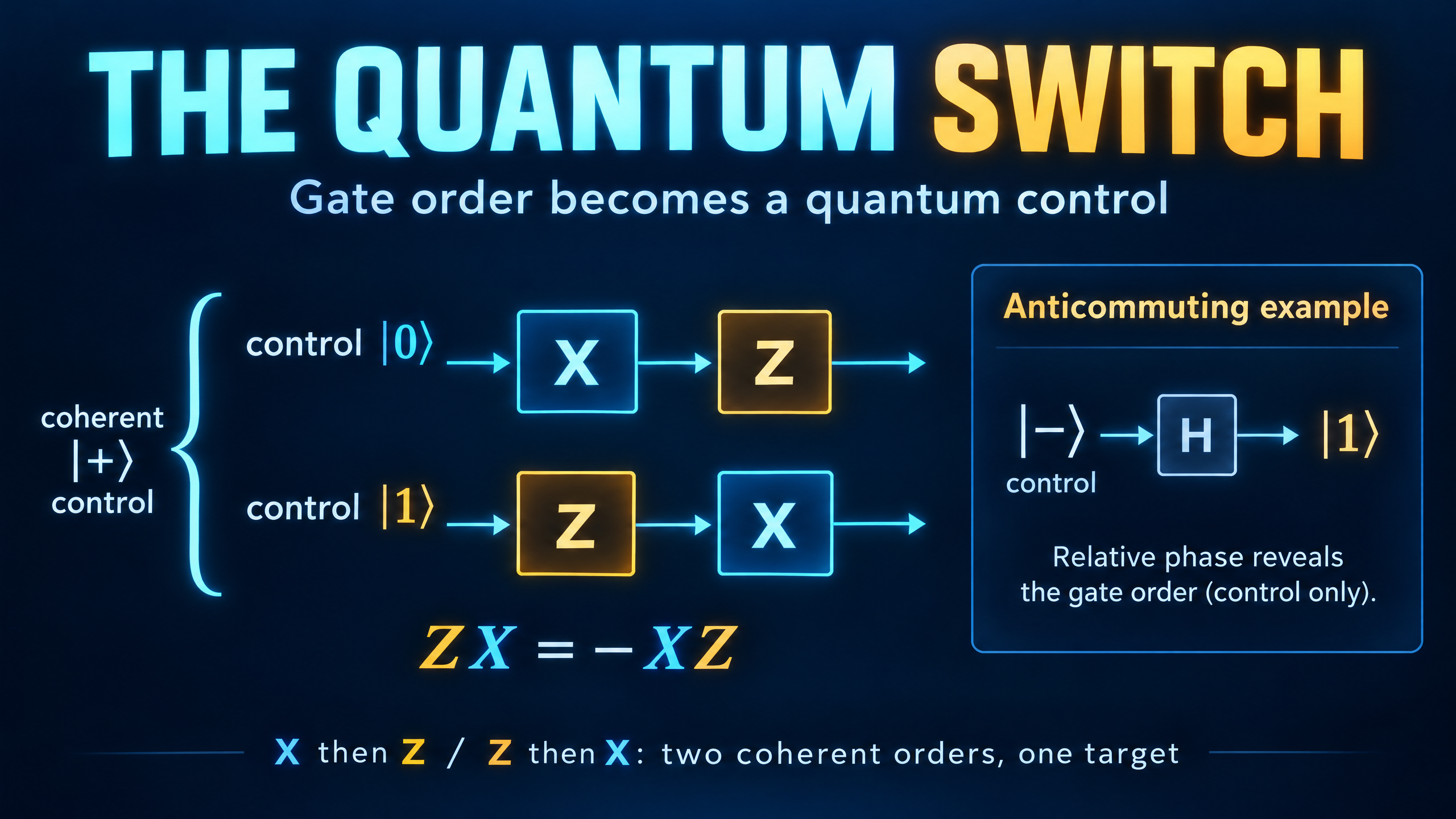
Apply X and then Z to a qubit. Now reverse their order. The two results differ by a minus sign, because ZX = -XZ.
If you run those two experiments separately and only examine the target qubit, that minus sign is a global phase. It cannot distinguish the outputs. But put the two orders into a coherent superposition, and the sign becomes a relative phase between control branches. Interference can reveal it.
That is the central idea behind a quantum switch: a control system coherently selects the order in which operations act on a target. Here we will derive its readout and check it with a small NumPy simulation.
Define the order before multiplying matrices
Let U and V be unitary gates on a target state |psi>. Use a separate control qubit and choose this convention:
- Control |0>: apply U first, then V. The target transformation is VU.
- Control |1>: apply V first, then U. The target transformation is UV.
Matrix products act from right to left. Keeping that convention explicit prevents an easy order-of-operations mistake.
With the control listed first in the tensor product, the joint switched transformation is
W = |0><0| tensor VU + |1><1| tensor UV.
Prepare the control in |+>. Before reading it out, the joint state is
(|0> tensor VU|psi> + |1> tensor UV|psi>) / sqrt(2).
The cover specializes these two histories to U = X and V = Z. They are alternative coherent orders acting on one target, not two target qubits or a classical choice between independent experiments.
Let the two orders interfere
Apply H to the control, then measure that control in the computational basis. The final joint state becomes
|0> tensor (VU + UV)|psi>/2 + |1> tensor (VU - UV)|psi>/2.
The sum is the anticommutator of V and U. The difference is their commutator, with the order convention [V,U] = VU - UV.
The readout probabilities are therefore
p0 = norm((VU + UV)|psi>)**2 / 4,
p1 = norm((VU - UV)|psi>)**2 / 4.
If the gates commute, VU = UV, so p1 is zero and the control always reads 0. If they anticommute, VU = -UV, so p0 is zero and the control always reads 1. These deterministic statements hold for any normalized target input under the corresponding operator identity.
There is an important promise hiding in that useful binary test. The gates must be guaranteed to fall into one of those two classes. Arbitrary gates can produce intermediate probabilities. A single outcome does not generally certify an operator identity.
Where the minus sign went
For X and Z, the state before the final H factors as
|-> tensor ZX|psi>.
The control has become |->, while the target carries the common operation ZX. The final H maps |-> to |1>, making the relative sign visible as a deterministic control result.
There is no contradiction with the rule that global phase is unobservable. A phase common to the entire joint state is still global. Here the sign appears between two components of a larger state, so it is relative.
Nor is this equivalent to tossing a coin to choose an order. If the control starts as a 50/50 classical mixture of |0> and |1>, the order branches have no coherence. After the controlled transformation and final H, the control reads 0 and 1 with equal probability. The interference signal is lost.
Simulate three cases in NumPy
We use control-first basis order |00>, |01>, |10>, |11>. The target input is (|0> + i|1>)/sqrt(2). Stacking the two target branches constructs W acting on the prepared input without explicitly building a four-by-four W matrix.
The third test uses U = X and V = Rz(pi/3), where
Rz(angle) = diag(exp(-i*angle/2), exp(i*angle/2)).
That pair is neither commuting nor anticommuting. It produces p0 = 0.75 and p1 = 0.25, rather than a deterministic class label.
import numpy as np

I = np.eye(2, dtype=complex)
X = np.array([[0, 1], [1, 0]], dtype=complex)
Z = np.diag([1, -1]).astype(complex)
H = np.array([[1, 1], [1, -1]], dtype=complex) / np.sqrt(2)
psi = np.array([1, 1j], dtype=complex) / np.sqrt(2)

def rz(angle):
    return np.diag([np.exp(-1j*angle/2), np.exp(1j*angle/2)])

def switch_probs(U, V):
    assert np.allclose(U.conj().T @ U, I)
    assert np.allclose(V.conj().T @ V, I)
    branches = np.r_[V @ U @ psi, U @ V @ psi] / np.sqrt(2)
    out = (np.kron(H, I) @ branches).reshape(2, 2)
    probs = np.sum(np.abs(out)**2, axis=1)
    formula = [np.linalg.norm((V@U + U@V) @ psi)**2 / 4,
               np.linalg.norm((V@U - U@V) @ psi)**2 / 4]
    assert np.allclose(probs, formula)
    assert np.isclose(probs.sum(), 1)
    return probs

cases = [("X, Z", X, Z, [0, 1]),
         ("Z, Z", Z, Z, [1, 0]),
         ("X, Rz(pi/3)", X, rz(np.pi/3), [0.75, 0.25])]
for name, U, V, expected in cases:
    p0, p1 = switch_probs(U, V)
    assert np.allclose([p0, p1], expected)
    print(f"{name}: p0={p0:.6f}, p1={p1:.6f}")
Expected output:
X, Z: p0=0.000000, p1=1.000000
Z, Z: p0=1.000000, p1=0.000000
X, Rz(pi/3): p0=0.750000, p1=0.250000
The code computes both branch products from known matrices. That is enough to test the interference algebra, but it is not an implementation that queries unknown physical gates only once each.
A matrix simulation is not a query-advantage experiment
A quantum switch is often discussed in the context of superposed causal orders. In a photonic realization, for example, spatial paths can coherently control the order in which gate devices act on a polarization target. The control must retain coherence so the histories can interfere.
For the promised commuting-versus-anticommuting task with otherwise unknown gates, the quantum-switch experiment described in the reference below uses one query to each gate. Its comparison with fixed-order circuits is a statement about that specific access model and promise, not a blanket speedup for every computation.
Our simulation makes no such resource claim. Known matrix products can be embedded in a conventional controlled operation. Merely simulating that joint unitary, or compiling known controlled products in a fixed-order circuit, does not by itself demonstrate a physical indefinite-causal-order resource. The relevant distinction concerns how the unknown gate operations are supplied and used.
Nothing here implies time travel or faster-than-light communication. The operational point is more modest and more useful: coherent alternatives can expose a relationship between operations that their separate target outputs hide.
Try changing the phase gate
Replace pi/3 in the third test with another angle. For this X and Rz(angle) family, the control probabilities are p0 = cos(angle/2)**2 and p1 = sin(angle/2)**2. Angle zero gives a commuting pair. Angle pi gives an anticommuting pair, up to the irrelevant overall phase of the Rz gate. Intermediate angles interpolate between the two.
This is a good programming check because it tests more than one favorable example. It also makes the conceptual lesson concrete: the control readout comes from interference between gate orders, not from observing an isolated global phase.
Further reading
Experimental Superposition of Orders of Quantum Gates, by Procopio and colleagues, derives the commutator and anticommutator readout, explains the promised query task, and describes a photonic implementation. Its physical resource accounting is distinct from the known-matrix simulation above.