Quantum Volume: What the Heavy Output Test Actually Measures
Calculate a heavy-output score in Python, distinguish ideal probabilities from measured samples, and see why one good histogram does not certify Quantum Volume.
A processor can have many qubits and still struggle to run a useful circuit. Gate errors, limited connectivity, readout errors, and compilation overhead all matter. Quantum Volume packages several of those effects into a particular random-circuit benchmark.
Its central question is surprisingly concrete: does the implemented circuit produce the outcomes that its ideal version considers more likely? Understanding that question is more useful than treating the final number as a universal ranking of quantum computers.
First choose a family of circuits
The Quantum Volume protocol uses randomized model circuits. For a square instance of size m, there are m qubits and m model layers. The layers contain random two-qubit unitaries, with qubit permutations arranging which qubits interact.
These are abstract model circuits. Compiling one onto a processor can add native gates and routing operations. The model depth m is not necessarily the depth of the final hardware circuit.
If the largest certified square size is m, the reported Quantum Volume is 2^m. For example, a certified size of four corresponds to Quantum Volume 16. That does not mean sixteen physical qubits were used, and it does not guarantee success for every possible circuit on four qubits.
The original Quantum Volume paper by Cross and colleagues defines the model circuits, their compilation, and the heavy-output test used to judge their execution.
What makes an output heavy?
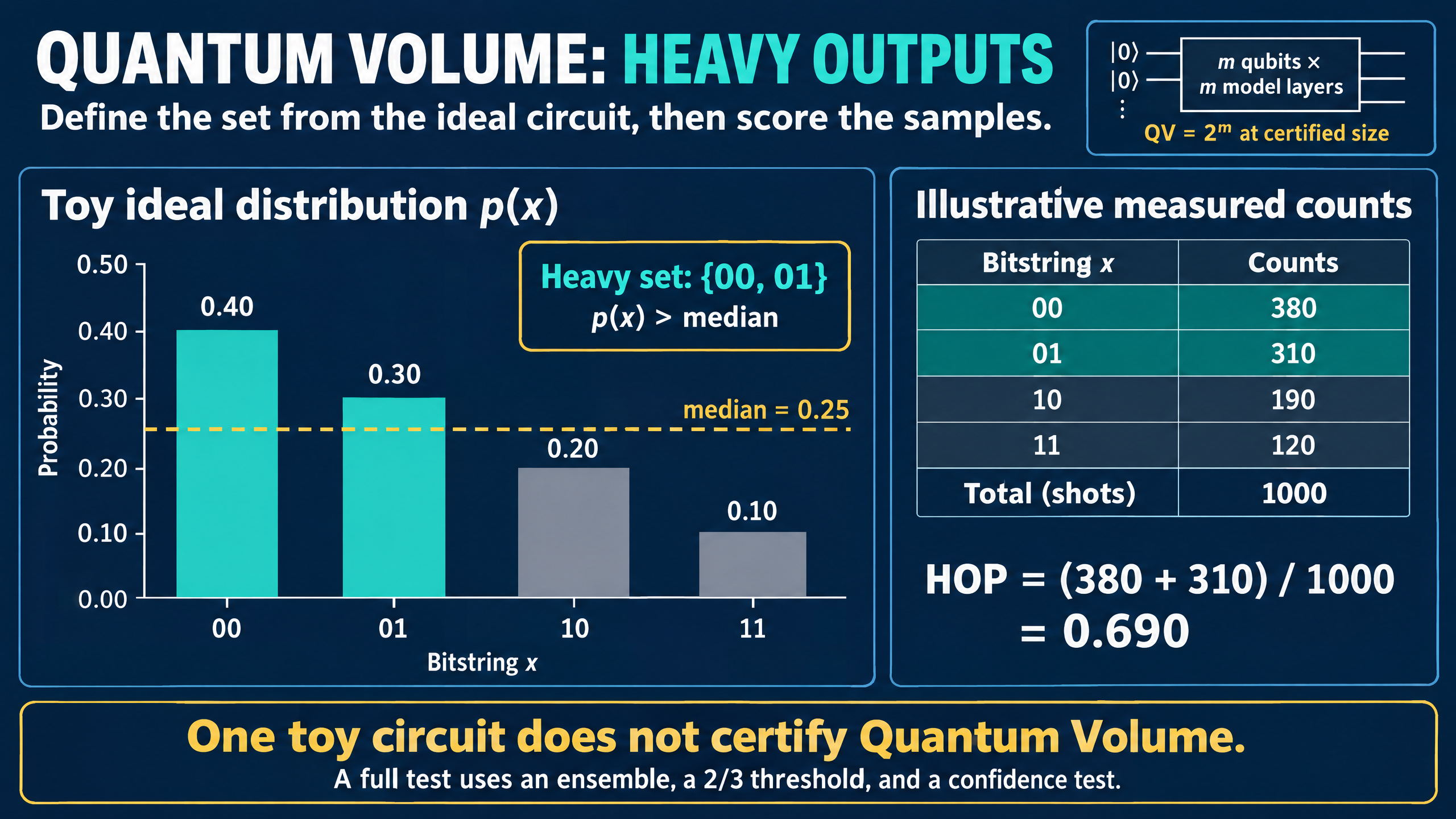
For one ideal circuit U, calculate the computational-basis outcome probabilities p_U(x). Find the median of those probabilities. The heavy set is:
H_U = {x : p_U(x) > median_y p_U(y)}
The comparison is strictly greater than the median. For generic random circuits without ties, half the bitstrings are heavy. They contain more than half of the ideal probability mass.
Now run the compiled circuit and collect samples. If its actual output distribution is q_U(x), the heavy-output probability is:
HOP = sum over x in H_U of q_U(x)
The ideal circuit defines the set. The experimental outcomes determine how much observed probability lands inside it. Recomputing the heavy set from the measured histogram would change the question and would not implement this test.
Score a small example in Python
Consider this illustrative two-qubit ideal distribution:
bitstring:  00    01    10    11
p(x):     0.40  0.30  0.20  0.10
Its median is 0.25, so the heavy set is {00, 01}. The ideal heavy-output probability is 0.70.
The code below uses a hypothetical measured histogram to calculate the score. It is classical postprocessing, not a random-circuit generator, a hardware experiment, or a Quantum Volume certification.
from statistics import median

ideal = {"00": 0.40, "01": 0.30, "10": 0.20, "11": 0.10}
cutoff = median(ideal.values())
heavy = {bits for bits, probability in ideal.items()
         if probability > cutoff}

def heavy_fraction(counts):
    if (not set(counts) <= set(ideal)
            or any(n < 0 for n in counts.values())
            or sum(counts.values()) <= 0):
        raise ValueError("Expected nonnegative counts for known outcomes")
    return sum(counts.get(bits, 0) for bits in heavy) / sum(counts.values())

measured = {"00": 380, "01": 310, "10": 190, "11": 120}
uniform = {bits: 250 for bits in ideal}
concentrated = {"00": 1000}

print(f"Ideal median: {cutoff:.2f}")
print("Heavy strings:", sorted(heavy))
print(f"Ideal HOP: {sum(ideal[x] for x in heavy):.3f}")
print(f"Measured HOP: {heavy_fraction(measured):.3f}")
print(f"Uniform HOP: {heavy_fraction(uniform):.3f}")
print(f"Concentrated HOP: {heavy_fraction(concentrated):.3f}")
Output:
Ideal median: 0.25
Heavy strings: ['00', '01']
Ideal HOP: 0.700
Measured HOP: 0.690
Uniform HOP: 0.500
Concentrated HOP: 1.000
In the measured example, 690 of 1,000 samples belong to the ideal heavy set. Uniform sampling puts half the probability there because this set contains two of the four bitstrings.
The final line is a useful warning. A distribution concentrated entirely on 00 scores one for this particular set, even though it is very different from the ideal distribution. Heavy-output probability is not a fidelity or a complete comparison of distributions.
That is not a valid shortcut to a benchmark result. The protocol requires an honest compiled implementation of the requested random circuit, not a simpler operation chosen merely to emit its heavy outputs.
Why 0.690 does not certify anything here
The benchmark's threshold is a mean heavy-output probability greater than 2/3 over an ensemble of random circuits, with a statistical confidence requirement. It is not a rule that one circuit with a sample score above 2/3 earns a Quantum Volume value. Nor does it mean that a majority of individual circuits must each pass that threshold.
The Qiskit Experiments Quantum Volume guide requires at least 100 circuit trials and applies a two-sigma confidence condition. An observed mean that barely exceeds 2/3 may still fail the confidence test.
There are two reasons to collect enough data: finite shots make each circuit's heavy fraction uncertain, and different random circuits have different heavy-output probabilities. Repeating one chosen circuit many times does not replace sampling the benchmark ensemble.
Our toy histogram deliberately leaves that ensemble and its confidence analysis out. It demonstrates how to compute a score, not how to report a processor's Quantum Volume.
Read the number with its scope attached
Quantum Volume captures the execution of a specific family of random circuits, including the effects of gates, connectivity, readout, and the compilation toolchain. Improvements in any of those can improve the result. The chosen physical qubits and compilation settings therefore belong alongside a reported value.
It does not certify every algorithm, compare execution speed, reveal all errors in a unitary, or by itself establish useful quantum advantage. Even matching computational-basis probabilities would not certify all quantum phases, and heavy-output probability contains less information than the full distribution.
The original protocol also needs classical ideal-circuit calculations to identify heavy outputs, which limits how far that exact verification approach can scale.
The practical habit is to keep three objects separate: the ideal probability distribution, the observed samples, and the ensemble-level acceptance test. Confusing any two makes an attractive benchmark number much easier to misread.