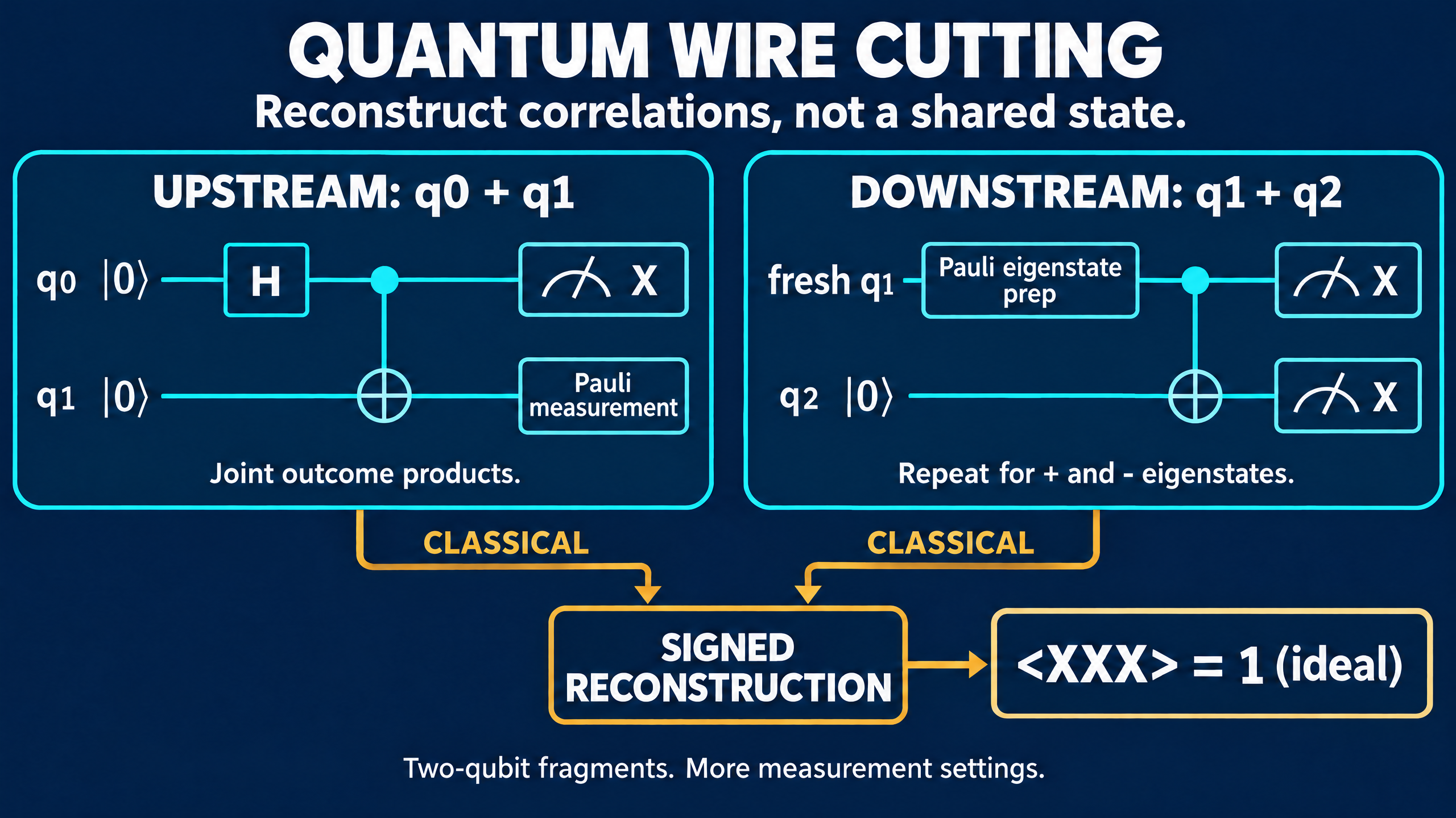
Quantum Wire Cutting: Rebuild a Correlation from Smaller Circuits
Cut a three-qubit GHZ circuit into two-qubit fragments, reconstruct its correlations with a signed Pauli sum, and see why fewer qubits require more experiments.
A wire in a quantum circuit carries more than a bit value. Its qubit may be entangled with the rest of the computation. Cutting that wire and preparing a fresh qubit in an ordinary guessed state will generally lose information.
Quantum wire cutting takes a different approach. Run several versions of smaller circuits, collect measurement statistics, then combine those statistics with signed weights. The goal is to reconstruct a requested result of the original circuit, not physically reconnect its quantum state.
A three-qubit example makes that distinction concrete.
Split a GHZ circuit into two fragments
Start in |000>. Apply H to q0, CNOT from q0 to q1, then CNOT from q1 to q2. The final state is the GHZ state:
(|000> + |111>) / sqrt(2)
Cut q1 between the two CNOTs. The upstream fragment contains q0 and q1 and prepares a Bell pair. The downstream fragment contains a newly prepared version of q1 and q2, initially in |0>, followed by the second CNOT. Each fragment uses only two qubits.
The original GHZ state has <XXX> = 1: measuring all three qubits in X gives a product of outcomes equal to +1. It also has <ZIZ> = 1 and <XIX> = 0. Here a label such as ZIZ means Z on q0, identity on q1, and Z on q2.
We will reconstruct these expectations from fragment data. The separate runs never need to hold a shared three-qubit GHZ state.
Keep the correlation at the cut
Suppose the requested observable is OA on q0, multiplied by OB on the downstream pair q1 and q2. For each P in {I, X, Y, Z}, obtain the upstream quantity
a_P = <OA tensor P>_upstream
For nonidentity P, this means measuring OA and P in the same upstream run and averaging their outcome products. Multiplying their separately averaged outcomes is not equivalent. The Bell pair, for instance, has <X tensor X> = 1 even though each individual X average is zero.
Next define f(sigma) as the downstream expectation of OB when its input q1 is prepared in state sigma and q2 starts in |0>. For P equal to X, Y, or Z, its eigenstate density matrices are
sigma_P,+ = (I + P) / 2
sigma_P,- = (I - P) / 2
Run the downstream circuit for these preparations and form
b_P = f(sigma_P,+) - f(sigma_P,-)
b_I = f(|0><0|) + f(|1><1|)
The identity contribution uses a sum, not a difference. I itself has trace two, so it is not a normalized state to prepare. The two Z eigenstates provide its contribution through linearity.
The reconstructed expectation is
<OA tensor OB> = (1/2) sum over P in {I,X,Y,Z} of a_P b_P
This follows from expanding the cut qubit's operator space in the Pauli basis. Crucially, the coefficients retain its correlations with q0. Using only that qubit's reduced density matrix would throw those correlations away.
The PennyLane circuit-cutting tutorial develops the measurement-and-preparation expansion behind this method. The six Pauli eigenstates used here are a transparent choice, not a claim of an optimal preparation scheme.
Reconstruct it with NumPy
This code evaluates the fragment statistics exactly using density matrices. It does not generate finite-shot samples or run on hardware. The small uncut simulation is included only as a reference check. Qubit labels run left to right in every tensor product.
import numpy as np

I = np.eye(2, dtype=complex)
X = np.array([[0, 1], [1, 0]], dtype=complex)
Y = np.array([[0, -1j], [1j, 0]], dtype=complex)
Z = np.diag([1, -1]).astype(complex)
zero = np.diag([1, 0]).astype(complex)
CX = np.array([[1, 0, 0, 0], [0, 1, 0, 0],
               [0, 0, 0, 1], [0, 0, 1, 0]], dtype=complex)

bell = np.array([1, 0, 0, 1], dtype=complex) / np.sqrt(2)
upstream = np.outer(bell, bell.conj())

def mean(state, observable):
    return float(np.trace(state @ observable).real)

def downstream(sigma, observable):
    state = CX @ np.kron(sigma, zero) @ CX.conj().T
    return mean(state, observable)

def reconstruct(OA, OB):
    total = 0.0
    for label, P in [("I", I), ("X", X), ("Y", Y), ("Z", Z)]:
        a = mean(upstream, np.kron(OA, P))
        if label == "I":
            b = downstream(zero, OB) + downstream(I - zero, OB)
        else:
            b = (downstream((I + P) / 2, OB)
                 - downstream((I - P) / 2, OB))
        total += a * b / 2
    return total

# Reference: continue the Bell pair with q2 in |0>.
psi = np.kron(I, CX) @ np.kron(bell, np.array([1, 0]))
uncut = np.outer(psi, psi.conj())

for label, OA, OB in [("XXX", X, np.kron(X, X)),
                      ("ZIZ", Z, np.kron(I, Z)),
                      ("XIX", X, np.kron(I, X))]:
    direct = mean(uncut, np.kron(OA, OB))
    stitched = reconstruct(OA, OB)
    print(f"{label}: uncut={direct:.6f}, cut={stitched:.6f}")
    assert np.isclose(direct, stitched)
Output:
XXX: uncut=1.000000, cut=1.000000
ZIZ: uncut=1.000000, cut=1.000000
XIX: uncut=0.000000, cut=0.000000
For XXX, the upstream X-X correlation is one, and the downstream responses to |+> and |-> are +1 and -1. Their difference is two. The factor one half then gives the reconstructed result of one.
This is a reconstruction of a number from multiple experiments. It does not mean either two-qubit fragment contains the original three-qubit state, or that one pair of fragment runs supplies one ordinary shot of the uncut circuit.
Fewer qubits, more experiments
The IBM wire-cutting guide follows the same broad workflow: partition the circuit, generate measurement and preparation experiments, run them, and reconstruct the desired expectation values.
The tradeoff is sampling cost. Differences and signed combinations can amplify statistical uncertainty. More cuts introduce more combinations of boundary data, and standard cutting schemes can incur an overhead exponential in the number of cuts. The precise cost depends on the decomposition, communication assumptions, and requested accuracy, as the Qiskit cutting documentation explains.
Smaller fragments may be easier to fit onto a processor and can reduce some circuit errors, but reconstruction does not automatically remove noisy preparation, gates, or measurements. A finite-shot estimate can even fall outside an observable's physical range because it is a signed statistical estimator. Clipping it changes the estimator and can introduce bias.
For this tiny GHZ circuit, classical calculation is simpler than any hardware experiment. Its purpose is to expose the mechanism, not demonstrate a speedup. Wire cutting becomes an engineering option when a useful partition fits the available hardware and its extra sampling and post-processing remain affordable. The question is not just whether a circuit can be split, but whether the reconstructed answer is worth the measurements it costs.