Qubit Leakage: When the State Leaves the Computational Subspace
A real qubit can occupy levels beyond |0> and |1>. A three-level NumPy example shows why leakage is not a bit flip, why renormalizing hides lost probability, and why detection is not recovery.
A qubit simulator usually gives each physical system exactly two basis states. A real device may have more. If some population moves outside the chosen |0>, |1> subspace, the problem is not just that the qubit has the wrong bit value. Part of its state has left the space in which the intended gates were defined.
That is leakage. A three-level example shows why it needs different bookkeeping from an ordinary bit flip, and why deleting the third entry from a simulation can give a misleading answer.
One intended qubit, more physical levels
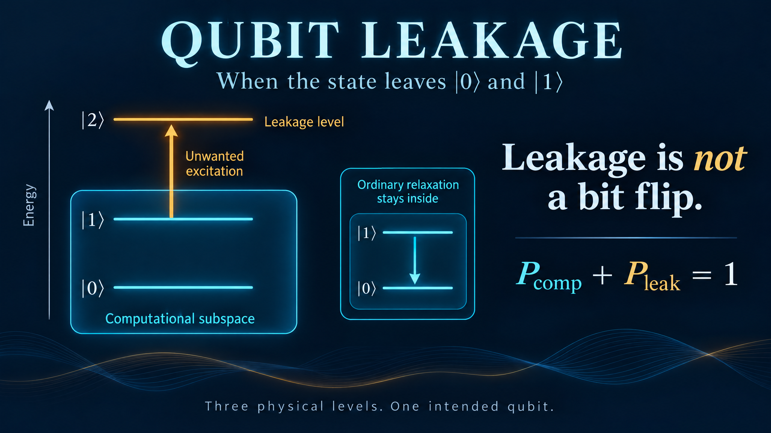
For a transmon, the two lowest energy levels usually define the computational subspace. Higher levels such as |2> still exist. Imperfect control can populate them, and some entangling operations intentionally use higher levels temporarily before returning population to the computational space.
An unwanted residual population outside that space is a leakage error. By contrast, a Pauli X error swaps |0> and |1> while remaining inside. Ordinary relaxation from |1> to |0> also stays inside, even though it can destroy the stored quantum information.
The distinction is about the destination, not simply whether an excitation was gained or lost. Our cover is a schematic level illustration, not an energy-scale plot.
For this tutorial, use the basis order |0>, |1>, |2> and the projector
P = diag(1, 1, 0).
For a normalized three-level density matrix rho,
P_comp = Tr(P rho) and P_leak = 1 - P_comp.
A state can have both computational and leakage components. It need not be entirely in one region or the other before a measurement.
An idealized coherent leakage rotation
Let an unwanted operation couple |1> and |2> while leaving |0> alone:
U(theta) = [[1,       0,             0],
            [0, cos(theta), -i*sin(theta)],
            [0, -i*sin(theta), cos(theta)]]
This is a unitary on the full three-level system. It is a deliberately simple model, not a calibrated transmon pulse simulation.
Start from the intended qubit state |+> = (|0> + |1>)/sqrt(2). The output is
(|0> + cos(theta)|1> - i*sin(theta)|2>)/sqrt(2).
Its leakage probability is sin(theta)**2 / 2. At theta equal to pi/3, the three level probabilities are 0.5, 0.125, and 0.375. We choose a large angle to make the bookkeeping visible, not to suggest a typical hardware error rate.
The full state is still pure and normalized. Leakage does not have to arise from an incoherent decay process.
Keep the missing probability visible
Projecting onto the computational space produces
rho_block = P rho P.
Its trace is the probability of finding the system in that subspace. In our example, the nonzero two-by-two block is
[[0.500, 0.250],
 [0.250, 0.125]]
The trace is 0.625, not one. That is useful information, not a numerical normalization error.
If an ideal measurement tells us the system is still in the computational subspace, the conditional state is rho_block divided by 0.625. Its |0>, |1> probabilities are then 0.8 and 0.2, and its off-diagonal entry is 0.4. It is not the original |+> state.
Simply deleting the leakage entry and renormalizing silently changes the question from "What happened in all runs?" to "What remains in the accepted runs?"
Verify the three-level calculation in NumPy
The code retains a three-by-three representation throughout. In rho_cond, the third row and column are zero; the first two entries give the conditioned qubit statistics.
import numpy as np

theta = np.pi / 3
c, s = np.cos(theta), np.sin(theta)
U = np.array([[1, 0, 0], [0, c, -1j*s], [0, -1j*s, c]], dtype=complex)
v = np.array([1, 1, 0], dtype=complex) / np.sqrt(2)
P = np.diag([1, 1, 0])

out = U @ v
pops = np.abs(out)**2
p_comp = float(np.vdot(out, P @ out).real)
projected = P @ out
rho_block = np.outer(projected, projected.conj())
rho_cond = rho_block / p_comp
cond_pops = np.real(np.diag(rho_cond))[:2]
coherence = rho_cond[0, 1]
restored = U.conj().T @ out

assert np.allclose(U.conj().T @ U, np.eye(3))
assert np.isclose(np.vdot(out, out).real, 1)
assert np.allclose(pops, [0.5, 0.125, 0.375])
assert np.isclose(p_comp, 0.625)
assert np.allclose(cond_pops, [0.8, 0.2])
assert np.isclose(coherence, 0.4)
assert np.allclose(restored, v)
assert not np.isclose(np.trace(rho_block).real, 1)

print(f"output probabilities: {pops[0]:.6f}, {pops[1]:.6f}, {pops[2]:.6f}")
print(f"computational probability: {p_comp:.6f}")
print(f"conditional computational probabilities: {cond_pops[0]:.6f}, {cond_pops[1]:.6f}")
print(f"conditional coherence rho[0,1]: {coherence.real:.6f} + {coherence.imag:.6f}j")
print(f"initial coherence rho[0,1]: {0.5:.6f}")
print(f"projected block trace: {np.trace(rho_block).real:.6f}")
print(f"U-dagger restores initial state: {np.allclose(restored, v)}")
print("all assertions passed")
Expected output:
output probabilities: 0.500000, 0.125000, 0.375000
computational probability: 0.625000
conditional computational probabilities: 0.800000, 0.200000
conditional coherence rho[0,1]: 0.400000 + 0.000000j
initial coherence rho[0,1]: 0.500000
projected block trace: 0.625000
U-dagger restores initial state: True
all assertions passed
The computational projection is trace-decreasing. Conditioning on its success is not a deterministic, trace-preserving qubit channel. The third level also belongs to the same physical system; it is not a separate extra qubit that we can simply trace out.
Reversibility is not a general repair strategy
In this noiseless model, applying the known U-dagger to the complete output restores the initial state. The code checks that before any leakage-detection measurement or postselection.
That does not mean a real leakage event can always be undone. An unknown operation, intervening noise, or a measurement that removes coherence between the subspaces changes the recovery problem. A flag that says "no leakage detected" is not proof that the surviving logical state is correct, as the biased conditional state already demonstrates.
Why hardware and error correction care
Leakage can persist across later gates. Those gates may behave differently on |2>, and interactions can spread errors to neighboring devices. A two-level Pauli noise model alone does not track that population or its effects.
Control methods such as DRAG pulse shaping suppress unwanted excitation of higher transmon levels. Leakage-removal operations address population that has already escaped. Resetting every device to |0> is not a general solution for data qubits, because it also erases the quantum state we wanted to preserve.
The programming lesson is straightforward: report leakage probability separately from the normalized statistics of surviving runs. A tidy two-entry state vector is not enough evidence that a physical qubit stayed inside its intended space.
Further reading
Google Quantum AI's explanation of leakage in error correction describes higher transmon levels, persistent leakage, and dedicated removal operations.
Leakage reduction in fast superconducting qubit gates explains how pulse bandwidth can drive unwanted transitions and how pulse shaping can reduce the problem.