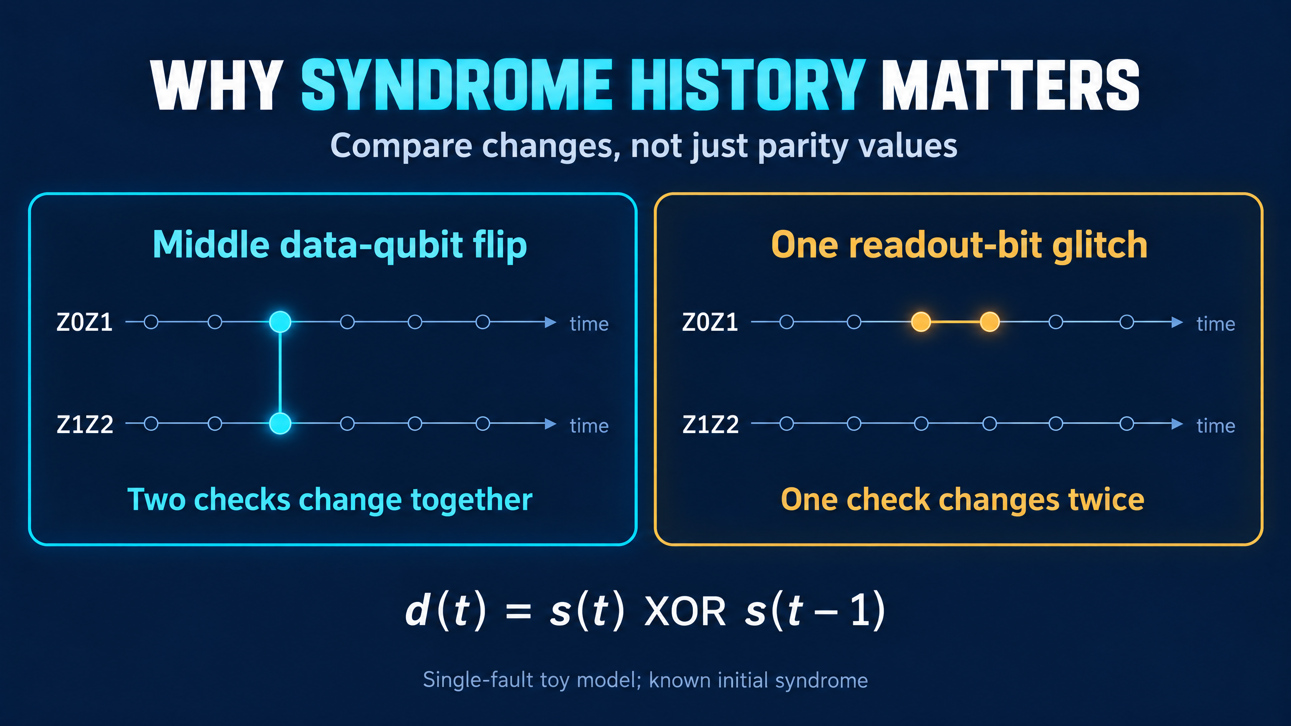
Repeated Syndromes: Why Error Correction Compares Changes
A persistent data error and a one-round readout glitch leave different trails. Use a small repetition-code example to turn repeated parity measurements into detection events.
A parity measurement reports an unexpected value. Should an error-correction system immediately flip a data qubit?
Not necessarily. The data might be wrong, or the reported measurement bit might be wrong. If every suspicious result triggers an immediate correction, a faulty detector can persuade the system to introduce an error that was not there before.
Repeated syndrome measurements give us another clue: how the record changes over time. A persistent data error and a brief readout glitch can produce different patterns of changes, even when a single measurement looks ambiguous.
Let's make that distinction concrete with three data qubits and six measurement rounds.
Two checks, without reading the logical state
Use the repetition-code state
alpha*|000> + beta*|111>,
with checks
S0 = Z0*Z1 and S1 = Z1*Z2.
Both codewords have eigenvalue +1 for both checks. Measuring these parities ideally does not distinguish |000> from |111>, so it does not reveal alpha and beta. We record +1 as syndrome bit 0 and -1 as bit 1. The two-bit syndrome is ordered (S0, S1).
A single X error on the middle data qubit anticommutes with both checks and changes the syndrome from 00 to 11. Unless something else happens, subsequent ideal measurements continue to report 11. The data error persists; the parity measurements do not repair it.
We are using this code only to illustrate bit-flip syndromes. These two Z-type checks do not protect an arbitrary logical state against phase errors.
Compare consecutive rounds
Let s(t) be the measured two-bit syndrome in round t. Define the detection-event bits as
d(t) = s(t) XOR s(t-1).
XOR is applied separately to each check. A detector bit is 1 when that check's reported value differs from its previous value. It flags a change, not simply a negative parity.
Assume the initial syndrome s(0) is known to be 00. A constant history of 11 after an error does not keep generating new events. Only the transition into 11 does.
The idea of using repeated measurements to separate persistent data changes from temporary measurement glitches is explained in PennyLane's surface-code introduction. We use a much smaller code here so every bit can be inspected.
Case 1: a middle-qubit flip before round 3
Suppose X1 occurs just before the third round. There are no other faults and we apply no corrections during the six-round window.
The measured syndromes are
00, 00, 11, 11, 11, 11.
Taking consecutive differences gives
00, 00, 11, 00, 00, 00.
There are two detection events: check 0 and check 1, both in round 3. On a picture with check position in one direction and time in the other, these are a spatial pair at the same time.
The repeated 11 values are useful evidence that the data's parity has changed. But counting every 1 in that raw history as a separate new data fault would badly misread the record.
Case 2: one reported bit is wrong
Now suppose the data have no error at all. Instead, check 0's reported bit flips only in round 3. Its next reported result is correct again.
The measured syndromes are
00, 00, 10, 00, 00, 00.
The detection events are
00, 00, 10, 10, 00, 00.
This time the pair is temporal: check 0 fires in rounds 3 and 4. One event marks the reported bit becoming wrong, and the other marks it returning to its correct value. Check 1 never changes.
The thumbnail contrasts exactly these two single-fault examples. Its bright dots represent detection events, not the raw syndrome values.
Generate both histories in NumPy
This is a classical simulation of Pauli-error bookkeeping, not a simulation of all quantum amplitudes. Each row of the data-error array describes the accumulated X-error pattern at one measurement round. A 1 means an odd number of X flips on that qubit relative to the ideal encoded state.
import numpy as np

def syndromes(x):
    # Check columns: S0 = Z0 Z1, S1 = Z1 Z2.
    return np.column_stack((x[:, 0] ^ x[:, 1],
                            x[:, 1] ^ x[:, 2]))

def detectors(measured):
    # Known initial syndrome 00; do not invent a final boundary.
    s = np.vstack((np.zeros((1, 2), dtype=np.uint8), measured))
    return s[1:] ^ s[:-1]

def locations(d):
    # Rounds are 1-based; check labels remain 0 and 1.
    return [(int(r) + 1, int(c)) for r, c in np.argwhere(d)]

x = np.zeros((6, 3), dtype=np.uint8)
x[2:, 1] = 1  # X1 occurs just before round 3 and persists.
s_data = syndromes(x)
d_data = detectors(s_data)

s_readout = np.zeros((6, 2), dtype=np.uint8)
s_readout[2, 0] = 1  # Only this reported bit is wrong.
d_readout = detectors(s_readout)

assert locations(d_data) == [(3, 0), (3, 1)]
assert locations(d_readout) == [(3, 0), (4, 0)]
assert np.array_equal(s_data[2:], np.ones((4, 2), dtype=np.uint8))
print("data events (round, check):", locations(d_data))
print("readout events (round, check):", locations(d_readout))
Expected output:
data events (round, check): [(3, 0), (3, 1)]
readout events (round, check): [(3, 0), (4, 0)]
Using XOR rather than subtraction keeps the results binary. It also reflects the fact that two X flips cancel in the accumulated Pauli frame.
The start and end of the record matter
We explicitly supplied s(0) = 00. Without a known starting value, the first measured syndrome cannot automatically be interpreted as a change from zero. Some checks can also have random initial outcomes in other preparation procedures, so their first valid comparisons must be defined accordingly.
At the end, we did not force the syndrome back to 00. The data error in case 1 is still present after round 6. Appending an artificial zero row would create events that no measurement established.
Real experiments can use final data-qubit measurements to construct additional boundary checks. Those are actual measurements with specified error models, not permission to assume the final state is clean.
A pattern is evidence, not a unique diagnosis
The two examples are easy to distinguish because we specified isolated faults in a deliberately simple model. Real measurement circuits have gate errors, ancilla errors, correlated faults, and boundaries. Their event patterns depend on details such as the extraction schedule and ancilla reset procedure.
Repeated-error-correction experiments process spatial and temporal correlations together. For example, Krinner and colleagues' experimental paper constructs syndrome changes across cycles and decodes them using a matching graph. Its circuit-specific correlations are richer than our one-round classical readout-flip model.
Even perfect syndrome measurements do not identify every physical error uniquely. X0 and X1X2 have the same two-check syndrome, while X0X1*X2 commutes with both checks and implements a logical bit flip. A decoder therefore combines the record with assumptions about which fault histories are likely. It cannot recover information the checks never revealed.
Our code generates detector records; it does not implement a decoder, claim fault tolerance, or guarantee correction of arbitrary noise.
The practical lesson is simple: a syndrome tells you about parity, while a syndrome history tells you about changes. Keeping those two records conceptually separate is the first step toward understanding why quantum error correction needs information in time as well as space.